Chapter 6 Simple Random Sampling
\(\DeclareMathOperator*{\argmin}{argmin}\) \(\newcommand{\var}{\mathrm{Var}}\) \(\newcommand{\bfa}[2]{{\rm\bf #1}[#2]}\) \(\newcommand{\rma}[2]{{\rm #1}[#2]}\) \(\newcommand{\estm}{\widehat}\)
Much of sample design theory for complex sample designs rests on the properties of the most simple of all designs: simple random sample without replacement (abbreviated SRSWOR or sometimes just SRS). We will investigate the properties of the SRSWOR later, but for the moment here is a working definition.
We have a population of size \(N\), from which we want to draw a sample of size \(n\) without replacement. i.e. each unit can only be drawn once, and \(n\) distinct units will be drawn from the population such that any sample of size \(n\) is equally likely.
6.1 Drawing a SRSWOR
One conceptual procedure for selecting a SRSWOR is the following:
- Select the first unit by randomly selecting with equal probability from the \(N\) units in the population
- Select the second unit by randomly selecting with equal probability from the \(N-1\) units which remain
- …
- Select the \(n^{\rm th}\) unit by randomly selecting with equal probability from the \(N-n+1\) units which remain
At the end we have a set of \(n\) distinct units in the sample, and \(N-n\) unselected units remaining in the population.
In practice we use other methods.
6.1.1 Taking a SRSWOR using a calculator
Most scientific calculators have a random number function – which generates a random number between 0 and 1 to 3 decimal places: e.g. 0.277 or 0.913. For populations \(N\) of a couple of hundred members, a SRSWOR can be drawn as follows:
- Generate a random number \(r\) between 0 and 1
- Calculate the number \(N\times r\) and no matter what the result round UP to the nearest whole number \(k\).
- Add the \(k^{\rm th}\) unit to the sample, unless it has already been selected.
- Go back to Step 1 and repeat until \(n\) units have been selected.
For example, if we want to select \(n=4\) units from a population of size \(N=8\) we proceed as follows:
- Generate \(r=0.675\) so \(Nr=(8)(0.675)=5.4\) round up to 6: select unit 6;
- Generate \(r=0.528\) so \(Nr=(8)(0.528)=4.2\) round up to 5: select unit 5;
- Generate \(r=0.161\) so \(Nr=(8)(0.161)=1.3\) round up to 2: select unit 2;
- Generate \(r=0.225\) so \(Nr=(8)(0.225)=1.8\) round up to 2: unit 2 already selected, so continue;
- Generate \(r=0.107\) so \(Nr=(8)(0.107)=0.9\) round up to 1: select unit 1.
So our sample is made up of units \(\{1, 2, 5, 6\}\).
6.1.2 Taking a SRSWOR using a spreadsheet
If we have all the units of a population listed in a spreadsheet such as Excel, it is straightforward to select a SRSWOR.
Using Excel:
- Insert a new column
- Fill each cell in the column with random numbers using the {} function. (To do this type {} in the first cell of the column, and then copy this into all of the cells in the column.)
- Make the values permanent by selecting the whole column, going Right-Click \(>>\) Copy, then Right-Click \(>>\) Paste Special. Select Paste Values and paste into the same column.
- Sort the whole spreadsheet by this new column (using Data \(>>\) Sort)
- Select the first \(n\) rows of the sorted spreadsheet and copy into a new spreadsheet.
This results in a SRSRWOR of size \(n\) from the population.
6.1.3 Taking a SRSWOR by scanning
It is very efficient in some computer languages to scan down the list of all the units of the population, and make a decision about whether to include each unit in turn. The algorithm below is a means of drawing a SRSWOR of \(n\) units from a list of size \(N\) by scanning the list once.
Set \(i=1\).
Generate a random number \(r\) between 0 and 1;
If \(r\leq \frac{n}{N}\) then select unit \(i\) into the sample and decrease \(n\) by 1: i.e. \(n \longleftarrow n-1\).
Decrease \(N\) by 1 and increase \(i\) by 1: i.e. \(N \longleftarrow N-1\) and \(i\longleftarrow i+1\)
If \(N>0\) goto 2.
else stop.
6.2 Notation: properties of populations and samples
6.2.1 Survey Population
A population is a set of members (called population units). A population can be either finite (e.g. all students enrolled at Victoria University at the start of the first trimester) or infinite (e.g. all passengers arriving at NZ ports). We will usually consider only finite populations, in which there is a well-defined (even if unknown) population size \(N\).
We give each unit (member) of the population a unique label \(i=1,\ldots,N\).
The population units have characteristics, (e.g. individuals have height, weight, income, age, sex). A given characteristic is represented by a variable \(Y\), and every (eligible) member \(i\) of the population has a value \(Y_i\) for that variable.
| Person label \(i\) | Gender | Highest Qual. | Age | Weekly hours worked | Weekly income | Marital Status | Ethnicity |
|---|---|---|---|---|---|---|---|
| 1 | female | school | 15 | 4 | 87 | never | European |
| 2 | female | vocational | 40 | 42 | 596 | married | European |
| 3 | male | none | 38 | 40 | 497 | married | Maori |
| 4 | female | vocational | 34 | 8 | 299 | never | European |
| 5 | female | school | 45 | 16 | 301 | married | European |
| 6 | male | degree | 45 | 50 | 1614 | married | European |
| 7 | female | none | 36 | 12 | 201 | other | European |
| … | … | … | … | … | … | … | … |
Recall that data items can be numerical (discrete or continuous), binary, categorical (nominal or ordinal).
Population parameters are characteristics of the whole population. e.g. if \(Y_i\) is the income of individual \(i\), then \[\begin{equation}\label{ytot} Y = \sum_{i=1}^N Y_i \end{equation}\] is the total income of all individuals in the population, and \[\begin{equation}\label{ybar} \bar{Y} = \frac{1}{N}\sum_{i=1}^N Y_i \end{equation}\] is the mean income in the population.
Table 6.2 contains a list of standard definitions for properties of populations. The values of the population parameters are in general unknown to us, and we must estimate them using the properties of samples.
| Quantity | Population | Sample |
|---|---|---|
| size | \(N\) | \(n\) |
| total | \(Y = \sum_{i=1}^N Y_i\) | \(y = \sum_{k=1}^n y_k\) |
| mean | \(\bar{Y} = \frac{1}{N}\sum_{i=1}^N Y_i\) | \(\bar{y} = \frac{1}{n}\sum_{k=1}^n y_k\) |
| variance | \(\sigma_Y^2=\frac{1}{N}\sum_{i=1}^N (Y_i-\bar{Y})^2\) | |
| adjusted variance | \(S_Y^2=\frac{1}{N-1}\sum_{i=1}^N (Y_i-\bar{Y})^2\) | \(s_y^2=\frac{1}{n-1}\sum_{k=1}^n (y_k-\bar{y})^2\) |
| adjusted variance for indicator variables | \(S_Y^2=\frac{N}{N-1}p(1-p)\) | \(s_y^2=\frac{n}{n-1}\widehat{p}(1-\widehat{p})\) |
| relative variance | \(V_Y^2=\frac{S_Y^2}{\bar{Y}^2}\) | \(v_y^2=\frac{s_y^2}{\bar{y}^2}\) |
| coefficient of variation | \(V_Y=\sqrt{V_Y^2}=\frac{S_Y}{\bar{Y}}\) | \(v_y=\sqrt{v_y^2}=\frac{s_y}{\bar{y}}\) |
| covariance | \(S_{XY}=\frac{1}{N-1}\sum_{i=1}^N (X_i-\bar{X})(Y_i-\bar{Y})\) | \(s_{xy}=\frac{1}{n-1}\sum_{k=1}^n (x_k-\bar{x})(y_k-\bar{y})\) |
| correlation coefficient | \(\rho_{XY}=\frac{S_{XY}}{S_XS_Y}\) | \(r_{xy}=\frac{s_{xy}}{s_xs_y}\) |
Binary Indicator Variables
Binary variables are often coded by indicator variables: which take the value 0 or 1 only. (e.g. \(Y_i=0\) if Male, \(Y_i=1\) if Female). The total of an indicator variable \[\begin{equation} Y = \sum_{i=1}^N Y_i = \text{Number of 1s} \end{equation}\] is just the number of units in the population for which the variable is 1 (e.g. the number of females in the population). The mean of an indicator variable is \[\begin{equation} \bar{Y} = \frac{1}{N}\sum_{i=1}^N Y_i = \frac{\text{Number of 1s}}{N} = P \end{equation}\] is then just the proportion of units \(P\) in the population that have the value 1 (e.g. the proportion of the population that is female).
6.2.2 Sample
A sample is a (non-empty) subset of the population containing \(n\) elements. In samples drawn without replacement each element is a distinct unit, whereas with replacement samples may contain repeated units.
We have a set of labels \(k=1,\ldots,n\) for each element of the sample, and these labels are of course different from the labels \(i=1,\ldots,N\) which we use to identify the population units.
We use lower case \(y_k\) to represent the value that the characteristic \(Y\) takes on the \(k\)th member of the sample. Thus if the \(k\)th member of the sample is the \(i\)th member of the population then \(y_k=Y_i\).
Sample statistics are characteristics of the sample. e.g. if \(y_k\) is the income of individual \(k\) in the sample, then \[\begin{equation} y = \sum_{k=1}^n y_k \end{equation}\] is the total income of all individuals in the sample, and \[\begin{equation} \bar{y} = \frac{1}{n}\sum_{k=1}^n y_k \end{equation}\] is the mean income in the sample.
A statistic is by definition a quantity which can be calculated from a sample of observations from a population. Certain statistics can be used as estimators of population parameters. For example, the sample mean may sometimes, but not always, be a good estimator of the population mean. However the sample total is never a good estimator of the population total (unless the ‘sample’ is actually a census).
An estimator \(\estm{T}\) is a particular type of statistic: its value is used to estimate the value of a population parameter \(T\).
Alongside the corresponding population properties, Table 6.2 contains a list of standard definitions for properties of samples.
The sampling fraction is the proportion of the population that has been sampled: \[\begin{equation} f = \frac{n}{N} \end{equation}\]
6.2.3 Sample Probabilities
The set of all possible samples that can be drawn under a particular sampling scheme is called the sample space \(\mathbb{S}\). Each possible sample \(s\) in the sample space has a known probability \(p(s)\).
Under simple random sampling there are \[\begin{eqnarray*} \binom{N}{n} &=& \frac{N!}{(N-n)!n!}\\ &=& \frac{N\times(N-1)\times(N-2)\times\ldots\times(N-n+1)}{ n\times(n-1)\times(n-2)\times\ldots\times 1} \end{eqnarray*}\] distinct possible samples of size \(n\) which can be drawn from a population of size \(N\), and each sample is equally likely. Therefore the probability of drawing any particular sample \(s\) is \[ p(s) = \frac{1}{\binom{N}{n}} = \frac{(N-n)!n!}{N!} \]
6.2.3.1 Example
Consider the following population \(U\):
| Unit, \(i\) | Value, \(Y_i\) |
|---|---|
| 1 | 0 |
| 2 | 1 |
| 3 | 3 |
| 4 | 5 |
| 5 | 6 |
| 6 | 9 |
There are \(N=6\) units in the population. Assume that we want to draw a SRSWOR of size \(n=2\). Then there are \(\binom{6}{2}=15\) possible samples: there are 6 ways to choose the first sample member, 5 ways to choose the second – so there are \(6\times5=30\) possible samples. However, the ordering of the elements in the sample is unimportant: sample \((i,j)\) is the same as sample \((j,i)\), hence we have \(\frac{30}{2}=15\) distinct samples.
| Sample | \(i_1\) | \(i_2\) | \(y_1=Y_{i_1}\) | \(y_2=Y_{i_2}\) | Sample Mean | Probability |
|---|---|---|---|---|---|---|
| 1 | 1 | 2 | 0 | 1 | 0.5 | \(\frac{1}{15}\) |
| 2 | 1 | 3 | 0 | 3 | 1.5 | \(\frac{1}{15}\) |
| 3 | 1 | 4 | 0 | 5 | 2.5 | \(\frac{1}{15}\) |
| 4 | 1 | 5 | 0 | 6 | 3.0 | \(\frac{1}{15}\) |
| 5 | 1 | 6 | 0 | 9 | 4.5 | \(\frac{1}{15}\) |
| 6 | 2 | 3 | 1 | 3 | 2.0 | \(\frac{1}{15}\) |
| 7 | 2 | 4 | 1 | 5 | 3.0 | \(\frac{1}{15}\) |
| 8 | 2 | 5 | 1 | 6 | 3.5 | \(\frac{1}{15}\) |
| 9 | 2 | 6 | 1 | 9 | 5.0 | \(\frac{1}{15}\) |
| 10 | 3 | 4 | 3 | 5 | 4.0 | \(\frac{1}{15}\) |
| 11 | 3 | 5 | 3 | 6 | 4.5 | \(\frac{1}{15}\) |
| 12 | 3 | 6 | 3 | 9 | 6.0 | \(\frac{1}{15}\) |
| 13 | 4 | 5 | 5 | 6 | 5.5 | \(\frac{1}{15}\) |
| 14 | 4 | 6 | 5 | 9 | 7.0 | \(\frac{1}{15}\) |
| 15 | 5 | 6 | 6 | 9 | 7.5 | \(\frac{1}{15}\) |
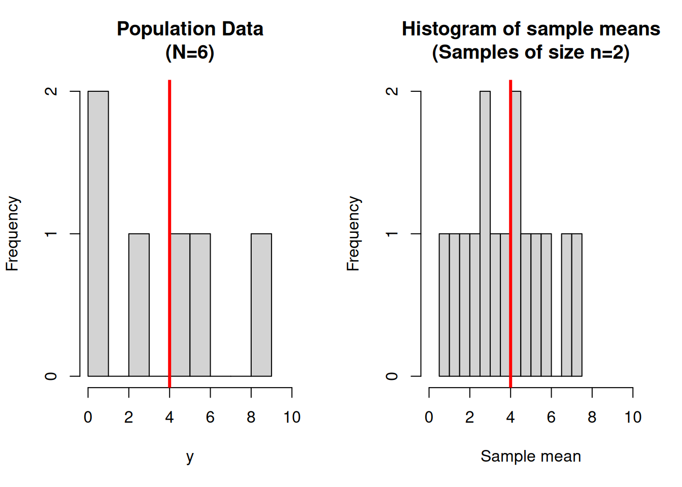
Figure 6.1: A population of size 6, and the means of all 15 samples of size 2. The mean of the population values, and the mean of all sample means are shown by a vertical line.
The population mean is \(\bar{Y}=4\), which can be compared with the 15 possible sample means \(\bar{y}\) listed in the table. The population variance is \(\sigma_Y^2=9.33\), and the standard deviation is \(\sigma_Y=3.06\).
The mean of the 15 sample means is \(\bar{\bar{y}}=4\) (equal to \(\bar{Y}\)), with standard deviation 2 (which is less than the population standard deviation). \end{quote}
The probability that any particular member \(i\) of the population ends up in the sample is called its inclusion probability, written \(\pi_i\). This probability must be nonzero for every unit in the survey population. In SRSWOR the inclusion probabilities are \[ \pi_i = \frac{n}{N} \] for every unit \(i\). In other words each unit has an equal chance of ending up in the sample. Not all sampling schemes have this property (e.g. in stratified samples the chances of being selected may vary between strata). In the example above the inclusion probabilities are \(\pi_i=\frac{2}{6}=\frac13\) for each unit.
The joint inclusion probabilities \(\pi_{ij}\) are the probabilities that both unit \(i\) and unit \(j\) are in the sample. These probabilities can sometimes be zero: for example consider a stratified random sample where we select one unit per stratum. If units \(i\) and \(j\) are in the same stratum then we have to have \(\pi_{ij}=0\), since if one is in the sample then the other can’t possibly be there too.
In SRSWOR the joint inclusion probabilities are \[ \pi_{ij} = \frac{n(n-1)}{N(N-1)} \qquad (i\neq j) \] for any pair of distinct units \(i,j\).
In the example above the inclusion probabilities are \(\pi_{ij}=\frac{2\times1}{6\times5}=\frac{1}{15}\) for any pair of units. is just the selection probability of the sample \(p(s)\) in each case. (This to be expected since each sample is exactly one pair of units.)
6.2.4 Sample Weights
In a general sampling scheme each unit \(i\) in the population has a known non-zero sample inclusion probability \(\pi_i\) and can be assigned a sample weight \[\begin{equation} w_i = \frac{1}{\pi_i} \end{equation}\] e.g. In a sample of \(n=2\) units from a population of size \(N=6\) under SRSWOR, the sample inclusion probability is \(\pi_i=\frac{2}{6}=\frac{1}{3}\) for each unit. The sample weights are therefore \[ w_i = \frac{1}{\pi_i} = 3 \] for each unit. i.e. each unit in the sample stands three units: itself and two others.
One way to think about this is that we replicate each sample member by its weight, and thereby create a synthetic population. We then use the properties of the synthetic population to estimate the parameters of the actual population.
Example
Consider the small population of 6 units again:
| Unit, \(i\) | Value, \(Y_i\) |
|---|---|
| 1 | 0 |
| 2 | 1 |
| 3 | 3 |
| 4 | 5 |
| 5 | 6 |
| 6 | 9 |
When we sample \(n=2\) units from this population of we might get units 2 and 4, each with weight 3.
| Unit, \(k\) | Value, \(y_k\) | Weight |
|---|---|---|
| 1 | 1 | 3 |
| 2 | 5 | 3 |
So we conceptually replicate each observation 3 times to create a synthetic population.
| Unit, \(i\) | Value, \(Y_i\) |
|---|---|
| 1 | 1 |
| 2 | 1 |
| 3 | 1 |
| 4 | 5 |
| 5 | 5 |
| 6 | 5 |
Certain of the properties of this synthetic population (e.g. the mean \(\bar{Y}=3\), and total \(Y=28\)) can be used to estimate properties of the actual population.
In many of Statistics NZ’s business surveys large businesses such as Telecom are always selected: i.e. they have a sample inclusion probability of 1. Their weights are therefore also 1: they represent themselves alone – which is appropriate since they are very different from all other businesses.
Small businesses may have much lower sampling inclusion probabilities e.g. \(\frac{1}{200}\), and consequently have much higher weights: 200. These businesses represent themselves and 199 others from the population.
We give a low sampling inclusion probability and therefore high weight to units which are similar to each other. Units which are rare and highly influential in estimation are given high sampling inclusion probabilities and low weights.
6.3 Estimation in SRSWOR
The principal population parameters that are usually of interest to us are the population total: \[\begin{equation} Y = \sum_{i=1}^N Y_i \end{equation}\] the population mean: \[\begin{equation} \bar{Y} = \frac{1}{N}\sum_{i=1}^N Y_i \end{equation}\] the adjusted population variance: \[\begin{equation} S_Y^2 = \frac{1}{N-1}\sum_{i=1}^N (Y_i-\bar{Y})^2 \end{equation}\] and the population variance: \[\begin{eqnarray} \sigma_Y^2 &=& \frac{1}{N}\sum_{i=1}^N (Y_i-\bar{Y})^2\\ \nonumber &=& \frac{N-1}{N}S_Y^2 \end{eqnarray}\]
For example, if we were taking a survey of incomes in a population, then we’d want to know the total income earned \(Y\), the mean income per head \(\bar{Y}\), and the variability of income between individuals \(S_Y\).
Example
Consider the survey of working hours and income from earlier: let’s treat these data as a population of size \(N=200\) from which we can sample. Note that we have added an extra column: an indicator variable which recodes the Highest Qualification column: \[ Y_i=\left\{\begin{array}{ll} 1& \text{if the person has post-school qualifications,}\\ 0& \text{otherwise} \end{array}\right. \]
| Personid | Gender | Qualification | Age | Hours | Income | Marital | Ethnicity | PostSchool | |
|---|---|---|---|---|---|---|---|---|---|
| 1 | 1 | female | school | 15 | 4 | 87 | never | European | 0 |
| 2 | 2 | female | vocational | 40 | 42 | 596 | married | European | 1 |
| 3 | 3 | male | none | 38 | 40 | 497 | married | Maori | 0 |
| 4 | 4 | female | vocational | 34 | 8 | 299 | never | European | 1 |
| 5 | 5 | female | school | 45 | 16 | 301 | married | European | 0 |
| 6 | 6 | male | degree | 45 | 50 | 1614 | married | European | 1 |
| 7 | 7 | female | none | 36 | 12 | 201 | other | European | 0 |
| 8 | … | … | … | … | … | … | … | … | … |
| 200 | 200 | male | school | 31 | 50 | 954 | never | European | 0 |
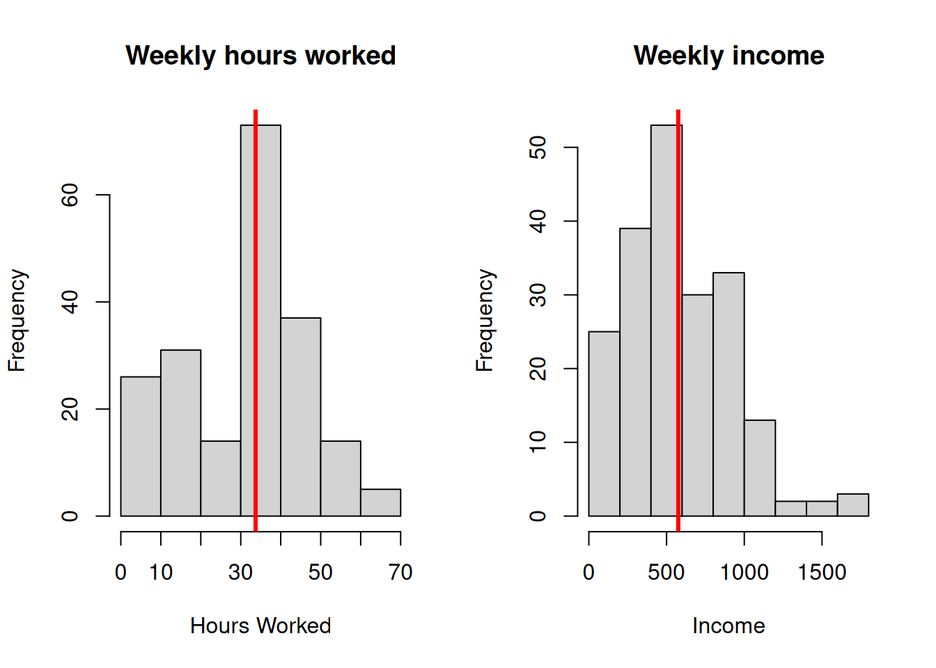
Figure 6.2: Distributions of Hours Worked and Income
The population parameters for working hours, income and post-school qualifications are:
| Parameter | Hours | Income | PostSchool |
|---|---|---|---|
| Pop. size \(N\) | 200.0000 | 200.0000 | 200.0000000 |
| Mean \(\bar{Y}\) | 33.7100 | 575.3600 | 0.4750000 |
| Total, \(Y\) | 6742.0000 | 115072.0000 | 95.0000000 |
| Adj. Variance \(S_Y^2\) | 261.0713 | 120137.6386 | 0.2506281 |
| Std. Deviation \(S_Y\) | 16.1577 | 346.6088 | 0.5006277 |
| Unadj. Variance $_Y^2 | 259.7659 | 119536.9504 | 0.2493750 |
Under SRSWOR we have estimators \(\estm{T}\) for each of these parameters \(T\): The SRSWOR estimator of the population total is \[\begin{equation} \estm{Y} = \frac{N}{n}\sum_{k=1}^n y_k = N\bar{y} \end{equation}\] the SRSWOR estimator of the population mean is the sample mean \(\bar{y}\): \[\begin{equation} \estm{\bar{Y}} = \bar{y} = \frac{1}{n}\sum_{k=1}^n y_k \end{equation}\] the SRSWOR estimator of the adjusted population variance is the sample variance \(s_y^2\): \[\begin{equation} \estm{S}_Y^2 = s_y^2 = \frac{1}{n-1}\sum_{k=1}^n (y_k-\bar{y})^2 \end{equation}\] and the SRSWOR estimator of the population variance is \[\begin{equation} \estm{\sigma}_Y^2 = \frac{N-1}{N}\estm{S}_Y^2 = \frac{N-1}{N}s_y^2 \end{equation}\] All four of these estimators are unbiased. That is to say, in the absence of non-sampling error, the mean value of their sampling distribution is equal to the population parameter of interest. In other words, if we take repeated samples and calculate the value of, say \(\estm{Y}\), then the values from those samples will scatter evenly around the true population total \(Y\).
For the special case where \(Y_i\) is an indicator variable the SRSWOR estimator of the population proportion \(P\) is the sample proportion \(\estm{p}\): \[\begin{equation} \estm{p} = \frac{1}{n}\sum_{k=1}^n I_k \end{equation}\] the SRSWOR estimator of the adjusted population variance is the sample variance \(s_y^2\) which takes the simple form: \[\begin{equation} \estm{S}_Y^2 = s_y^2 = \frac{n}{n-1}\estm{p}(1-\estm{p}). \end{equation}\]
Example continued
We have drawn a SRSWOR of \(n=20\) from the population of \(N=200\) people.
The probability of selection of each sample member is \[ \pi_k = \frac{n}{N}=\frac{20}{200} = 0.10 \] which is also the sampling fraction \(f=10\%\). The weight of each sample member is \[ w_k = \frac{1}{\pi_k} = \frac{N}{n}=\frac{200}{20} = 10 \] i.e. each person stands for his/herself and 9 others in the population.
| SampleID | Personid | Gender | Qualification | Age | Hours | Income | Marital | Ethnicity | PostSchool | Weight | |
|---|---|---|---|---|---|---|---|---|---|---|---|
| 57 | 1 | 57 | male | vocational | 40 | 39 | 525 | previously | Maori | 1 | 10 |
| 132 | 2 | 132 | female | vocational | 44 | 48 | 743 | married | European | 1 | 10 |
| 141 | 3 | 141 | female | degree | 23 | 45 | 658 | never | other | 1 | 10 |
| 86 | 4 | 86 | female | vocational | 35 | 40 | 501 | previously | Maori | 1 | 10 |
| 67 | 5 | 67 | female | vocational | 41 | 17 | 18 | married | European | 1 | 10 |
| 156 | 6 | 156 | male | vocational | 37 | 40 | 819 | married | European | 1 | 10 |
| 138 | 7 | 138 | female | none | 32 | 40 | 406 | married | European | 0 | 10 |
| 20 | 8 | 20 | female | none | 34 | 25 | 386 | other | European | 0 | 10 |
| 116 | 9 | 116 | female | degree | 36 | 40 | 925 | previously | European | 1 | 10 |
| 62 | 10 | 62 | female | degree | 28 | 50 | 544 | married | European | 1 | 10 |
| 151 | 11 | 151 | male | vocational | 18 | 40 | 1099 | other | European | 1 | 10 |
| 152 | 12 | 152 | female | school | 18 | 17 | 255 | never | European | 0 | 10 |
| 163 | 13 | 163 | female | vocational | 25 | 25 | 409 | never | Maori | 1 | 10 |
| 197 | 14 | 197 | male | degree | 26 | 50 | 1789 | never | European | 1 | 10 |
| 122 | 15 | 122 | male | vocational | 32 | 38 | 562 | married | European | 1 | 10 |
| 121 | 16 | 121 | female | vocational | 21 | 40 | 830 | other | European | 1 | 10 |
| 155 | 17 | 155 | female | vocational | 26 | 42 | 431 | married | European | 1 | 10 |
| 97 | 18 | 97 | female | vocational | 34 | 40 | 615 | never | European | 1 | 10 |
| 10 | 19 | 10 | male | school | 37 | 50 | 533 | previously | European | 0 | 10 |
| 165 | 20 | 165 | female | none | 45 | 40 | 439 | never | European | 0 | 10 |
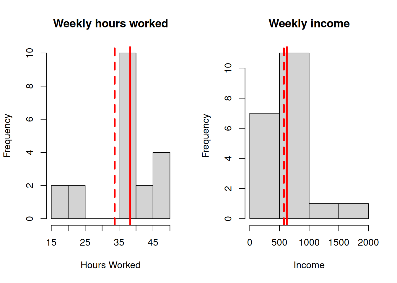
Figure 6.3: Sample distributions of Hours Worked and Income (true population mean shown as a dashed line)
The sample statistics for working hours and income are:
| Parameter | Hours | Income | PostSchool |
|---|---|---|---|
| Sample. size \(n\) | 20.000000 | 20.0000 | 20.0000000 |
| Mean \(\bar{y}\) | 38.300000 | 624.3500 | 0.7500000 |
| Adj. Variance \(s_y^2\) | 97.273684 | 133580.3447 | 0.1973684 |
| Std. Deviation \(s_y\) | 9.862742 | 365.4864 | 0.4442617 |
Our best estimates of the mean numbers of hours worked and income earned are 38.3 hours and $624.35 respectively (compare these to the true values of 33.71 hours and $575.36). We estimate the proportion of people with post-school qualifications to be 75% (compared to the true value of 47.5%).
Note that the sample has missed people working very short and very long hours, and that even though the estimate of the mean is close to the population value (the dashed line in the histogram), the sample variance \(s_y^2\) is much smaller than the population variance \(S_Y^2\). This sample also has a higher proportion of people with post-school qualifications than is the case in the general population. \end{quote}
6.3.1 Using sample weights to make estimates in SRSWOR
To estimate the total of a quantitative variable, sum up the values of the variable, weighted by the sample weights: \[\begin{equation} \estm{Y} = \sum_{k=1}^n w_k y_k = \sum_{k=1}^n y_k \frac{N}{n} = \frac{N}{n}\times \sum_{k=1}^n y_k = N\bar{y} \end{equation}\] This estimator is sometimes called the rate-up estimator – we take the sample total \(\sum_ky_k\) and ‘rate it up’ to the population by multiplying by the factor \(N/n\).
Example. To estimate the total income earned by the population as a whole during a single week multiply each value of income earned by the sample weight, and sum up the result. For SRSWOR since the weights are all the same, an alternative is to multiply the sample mean by the population size: \(N\bar{y}=(200)(624.35)=\$124870\) (true value $120138).
To estimate a mean, make an estimate of the total and divide through by the population size: \[\begin{equation} \estm{\bar{Y}} = \frac{\estm{Y}}{N} = \frac{1}{N}\sum_{k=1}^n w_k y_k = \frac{1}{N}\sum_{k=1}^n \frac{N}{n} y_k = \frac{1}{n}\sum_{k=1}^n y_k = \bar{y} \end{equation}\] i.e. in SRSWOR the estimate of the population mean is just the sample mean.
To estimate the total number of people in a certain category, add up the weights multiplied by an indicator variable \(y_k\): \[ y_k = \left\{\begin{array}{ll} 1,\ &\text{if unit $k$ is in the category}\\ 0, &\text{otherwise} \end{array}\right. \] which is the same as simply summing up the weights of survey respondents in that category: \[\begin{equation} \estm{Y} = \sum_{k=1}^n w_k y_k = \sum_{k\in \text{Category}} w_k = \sum_{k\in \text{Category}} \frac{N}{n} = \frac{N}{n}\times\text{(\# in the category in the sample)} \end{equation}\]
Example. to estimate the number of people with post-school qualifications, add up the weights for the sample members who have a post-school qualification. There are 15 such people, each with weight 10, so our estimate of the number of people with a post-school qualification is 150. We estimate that the proportion of people in the population with post-school qualifications is 150/200 = 75% (true proportion 47.5%).
The number of males in the sample is 6, each with weight 10, so we estimate that there are 60 males in the population.
To estimate the proportion of population members in a certain category we can either divide our estimate of the total number by the population size \(N\), or simply use the sample proportion as an estimate of the population proportion: the result is the same: \[\begin{equation} \estm{p} = \frac{\estm{Y}}{N} = \frac{1}{N}\frac{N}{n}\times\text{(\# in the category)} = \frac{1}{n}\times\text{(\# in the category)} = \text{sample proportion} \end{equation}\]
Example. We estimate that the proportion of males in the population is 60/200 = 30%. Alternatively the sample proportion is just \(\bar{y}=6/20=30\%\) (Note – the true proportion is 46.5%).
6.4 Sampling Errors
Sampling theory gives us formulae of the variance of the estimators in the previous section. We will only be concerned with the variances of the estimators for the population total and population mean.
These variances are \[\begin{eqnarray} \bfa{Var}{\estm{Y}} &=& N^2\left(1-\frac{n}{N}\right)\frac{S_Y^2}{n}\\ \bfa{Var}{\estm{\bar{Y}}} &=& \left(1-\frac{n}{N}\right)\frac{S_Y^2}{n} \end{eqnarray}\] and for estimates of the population proportion the variance is \[\begin{eqnarray} \bfa{Var}{\estm{p}} &=& \left(1-\frac{n}{N}\right)\frac{P(1-P)}{n} \end{eqnarray}\]
These formulae contain the finite population correction \[\begin{equation} \text{fpc} = 1-\frac{n}{N} = 1-f \end{equation}\] a factor which often appears in formulae in survey sampling. For small sampling fractions (i.e. small \(f=n/N\)) the fpc is approximately 1, and can be neglected. However, as \(n\) approaches \(N\) the fpc becomes closer and closer to zero. If we perform a census \(n=N\) then the fpc is zero and the variances of the estimators of \(Y\) and \(\bar{Y}\) are also zero. This is as it should be since there is no uncertainty about the true values of \(Y\) and \(\bar{Y}\) when we carry out a census: a census has no sampling error.
The formulae for the variances given above contain \(S_Y^2\): the adjusted population variance. This is a population parameter, and is unknown to us. However we can use the sample variance \(s_y^2\) to get an estimate of these variances: \[\begin{eqnarray} \bfa{\mbox{$\widehat{\bf Var}$}}{\estm{Y}} &=& N^2\left(1-\frac{n}{N}\right)\frac{s_y^2}{n}\\ \bfa{\mbox{$\widehat{\bf Var}$}}{\estm{\bar{Y}}} &=& \left(1-\frac{n}{N}\right)\frac{s_y^2}{n} \end{eqnarray}\] For proportions the corresponding expression is \[\begin{eqnarray} \bfa{\mbox{$\widehat{\bf Var}$}}{\estm{p}} &=& \left(1-\frac{n}{N}\right)\frac{\estm{p}(1-\estm{p})}{n-1} \end{eqnarray}\]
6.5 Confidence Intervals
The central limit theorem states that the distribution of sums and means of large samples of independent observations from a probability distribution are normally distributed.
In particular, if \(\estm{T}\) is an unbiased estimator of the population parameter \(T\) then (for sufficiently large sample sizes \(n\)) \(\estm{T}\) is Normally distributed with mean \(T\) and variance \(\bfa{Var}{\estm{T}}\).
This fact allows us to construct confidence intervals for our estimates.
The standard deviation of the sampling distribution of \(\estm{T}\) is called the standard error of the estimator \(\estm{T}\): \[\begin{equation} \bfa{SE}{\estm{T}} = \sqrt{\bfa{Var}{\estm{T}}} \end{equation}\] We can use the standard error to construct, say, a 95% confidence interval for the population parameter \(T\) in the usual way: \[\begin{equation} \text{95\% CI for $T$} = \estm{T}\pm 1.96\times\bfa{SE}{\estm{T}} \end{equation}\]
Example continued
Let’s construct a confidence interval for the population total weekly income using the SRS of size 20.
The sample statistics are \(n=20\), \(\bar{y}=624.35\), \(s_y^2=133580.34\), giving an estimate of the population total of \[\begin{eqnarray*} \estm{Y} &=& \frac{N}{n}\sum_{k=1}^n y_k = N\bar{y}\\ &=& 200\times 624.35 = 124870 \end{eqnarray*}\] and a standard error of \[\begin{eqnarray*} \bfa{SE}{\estm{Y}} &=& \sqrt{\bfa{Var}{\estm{Y}}} = \sqrt{N^2\left(1-\frac{n}{N}\right)\frac{s_y^2}{n}}\\ &=& \sqrt{200^2\left(1-\frac{20}{200}\right)\frac{133580.34}{20}}\\ &=& \sqrt{240445612} = 15506 \end{eqnarray*}\] This gives a margin of error for 95% confidence of: \[\begin{eqnarray*} \bfa{MOE}{\estm{Y}} &=& Z\times\bfa{SE}{\estm{Y}}\\ &=& 1.96\times 15506 = 30392 \end{eqnarray*}\] and hence a 95% confidence interval of \[\begin{eqnarray*} \estm{Y} \pm \bfa{MOE}{\estm{Y}} &=& 124870 \pm 30392\\ &=& (94478, 155262)\\ &=& (94500, 155300) \end{eqnarray*}\] This confidence interval is rather wide because the population is very variable, and a sample size of 20 is too small to give a good estimate. (Note – The true total value is 115072.)
6.6 Quality of Estimates
The precision of an estimate can be characterised by the relative standard error (RSE). This is defined: \[\begin{equation} \bfa{RSE}{\estm{T}} = \frac{\bfa{SE}{\estm{T}}}{\bfa{E}{\estm{T}}} \end{equation}\] i.e. it measures how big the standard error is, compared to the estimate itself. The RSE is a particular case of a coefficient of variation (CV), which is the standard deviation of a quantity divided by its mean. Usually CV’s are only useful for quantities which are strictly positive.
In general we don’t know the values of the standard error \(\bfa{SE}{\estm{T}}\) or of the mean of the estimator \(\bfa{E}{\estm{T}}\), but we can replace them as usual by estimates from our sample.
Example continued
The estimate of the population total is \(\estm{Y}=124870\), with a standard error of 15506. Thus the RSE is \[ \bfa{RSE}{\estm{Y}} = \frac{\bfa{SE}{\estm{Y}}}{\estm{Y}} = \frac{15506}{124870} = 0.12 = 12\% \] This RSE of 12% indicates a that the estimate is not of particularly high quality (we prefer RSEs close to 5% or 1% in general).
Let’s construct a confidence interval for the population mean weekly income using the SRS of size 20.
As before the sample statistics are \(n=20\), \(\bar{y}=624.35\), \(s_y^2=133580.34\), giving an estimate of the population mean of \[\begin{eqnarray*} \estm{\bar{Y}} &=& \frac{1}{n}\sum_{k=1}^n y_k = \bar{y}\\ &=& 624.35 \end{eqnarray*}\] and a standard error of \[\begin{eqnarray*} \bfa{SE}{\estm{\bar{Y}}} &=& \sqrt{\bfa{Var}{\estm{\bar{Y}}}} = \sqrt{\left(1-\frac{n}{N}\right)\frac{s_y^2}{n}}\\ &=& \sqrt{\left(1-\frac{20}{200}\right)\frac{133580.34}{20}}\\ &=& \sqrt{6011.1} = 77.5 \end{eqnarray*}\] This gives a margin of error for 95% confidence of: \[\begin{eqnarray*} \bfa{MOE}{\estm{\bar{Y}}} &=& Z\times\bfa{SE}{\estm{\bar{Y}}}\\ &=& 1.96\times 77.5 = 151.9 \end{eqnarray*}\] and hence a 95% confidence interval of \[\begin{eqnarray*} \estm{\bar{Y}} \pm \bfa{MOE}{\estm{\bar{Y}}} &=& 624.4 \pm 151.9\\ &=& (472.5, 776.3)\\ &=& (470,776) \end{eqnarray*}\] and an RSE of \[ \bfa{RSE}{\estm{\bar{Y}}} = \frac{\bfa{SE}{\estm{\bar{Y}}}}{\estm{\bar{Y}}} = \frac{77.5}{624.4} = 0.12 = 12\% \] It’s no coincidence that this is also 12%: a total and mean of the same variable will always have the same RSE.
Finally let’s repeat this procedure for the proportion of people with a post-school qualification. The relevant sample statistics are \(n=20\), and the sample proportion \(\estm{p}=\bar{y}=0.75\), giving an estimate of the population proportion of \[\begin{eqnarray*} \estm{p} &=& \bar{y} = \frac{15}{20} = 0.75 \end{eqnarray*}\] and a standard error of \[\begin{eqnarray*} \bfa{SE}{\estm{p}} &=& \sqrt{\bfa{Var}{\estm{p}}} = \sqrt{\left(1-\frac{n}{N}\right)\frac{\estm{p}(1-\estm{p})}{n-1}}\\ &=& \sqrt{\left(1-\frac{20}{200}\right)\frac{(0.75)(0.25)}{19}}\\ &=& \sqrt{0.00888} = 0.094 \end{eqnarray*}\] This gives a margin of error for 95% confidence of: \[\begin{eqnarray*} \bfa{MOE}{\estm{p}} &=& Z\times\bfa{SE}{\estm{p}}\\ &=& 1.96\times 0.094 = 0.185 \end{eqnarray*}\] and hence a 95% confidence interval of \[\begin{eqnarray*} \estm{p} \pm \bfa{MOE}{\estm{p}} &=& 0.75 \pm 0.185\\ &=& (0.57,0.94)\\ &=& (57\%,94\%) \end{eqnarray*}\] RSEs are not usually calculated for estimates of proportions: it is sufficient to quote the SE. In this case an SE of \(0.094\) or 9.4% is not very good. We really need a larger sample size for this and the earlier estimates.
Note. The above calculations for proportions are easily modified to give confidence intervals for total counts of individuals in a population with a particular property, since \(Y=Np\), and hence \(\widehat{Y}=N\widehat{p}\).
Thus in the above example the proportion of people with a post-school qualification is \(\widehat{p}=0.75\), so our estimate of the total number of people with a post-school qualification is \[ \widehat{Y} = N\widehat{p} = (200)(0.75) = 150 \] with a standard error of \[\begin{eqnarray*} \bfa{SE}{\estm{Y}} = N\bfa{SE}{\estm{p}} &=& N\sqrt{\bfa{Var}{\estm{p}}} = \sqrt{N^2\left(1-\frac{n}{N}\right)\frac{\estm{p}(1-\estm{p})}{n-1}}\\ &=& \sqrt{200^2\left(1-\frac{20}{200}\right)\frac{(0.75)(0.25)}{19}}\\ &=& 18.8 \end{eqnarray*}\] This gives a margin of error for 95% confidence of: \[\begin{eqnarray*} \bfa{MOE}{\estm{Y}} &=& Z\times\bfa{SE}{\estm{Y}}\\ &=& 1.96\times 18.8 = 36.8 \end{eqnarray*}\] and hence a 95% confidence interval of \[\begin{eqnarray*} \estm{Y} \pm \bfa{MOE}{\estm{Y}} &=& 150 \pm 37\\ &=& (113,187) \end{eqnarray*}\] and an RSE of \[ \bfa{RSE}{\estm{{Y}}} = \frac{\bfa{SE}{\estm{{Y}}}}{\estm{{Y}}} = \frac{18.8}{150} = 0.13 = 13\% \]
6.7 Sample Size Calculations
In the previous example we saw that the sample size was too small to give a good estimate. In the planning stage of a survey we almost always calculate the sample size that will be required to gain a specific accuracy. Such calculations are a crucial part of planning, and determine whether the survey can reach its objectives given the constraints of money and time.
6.7.1 Estimation of means
The required accuracy is usually specified in terms of a desired RSE or a desired margin of error. In general a confidence interval for a population mean takes the form \[ \text{CI} = \estm{\bar{Y}} \pm \bfa{MOE}{\estm{\bar{Y}}} \] For example for SRSWOR and the estimation of the population mean we have \[\begin{eqnarray*} \bfa{MOE}{\estm{\bar{Y}}} &=& Z\times\bfa{SE}{\estm{\bar{Y}}} \\ &=& Z\sqrt{\bfa{Var}{\estm{\bar{Y}}}}\\ &=& Z\sqrt{\left(1-\frac{n}{N}\right)\frac{S_y^2}{n}}\\ &=& Z\sqrt{\left(1-\frac{n}{N}\right)}\frac{S_y}{\sqrt{n}} \end{eqnarray*}\] In this formula we have
- \(m=\bfa{MOE}{\estm{\bar{Y}}}\) – we specify this, our desired MOE;
- \(Z\) = normal quantile for the appropriate level of confidence – we choose this: usually \(Z=1.96\) for 95% confidence;
- \(N\) = population size: this is usually known, or we have some estimate;
- \(S_Y^2\) = population variance – we estimate this from previous data (in the planning stages of a survey we have no sample to estimate \(S_Y^2\));
- \(n\) = sample size – this is what we want to deduce.
If \(N\) is large enough the fpc can be neglected, and the MOE formula becomes \[ m = Z\times \frac{S_Y}{\sqrt{n}} \] which can be rearranged to give \[\begin{equation} n' = \left(\frac{Z}{m}\right)^2 S_Y^2 \end{equation}\] We denote this sample size \(n'\), and note that it ignores the finite population correction. We can modify this first estimate of the sample size to take account of the fpc as follows: \[\begin{equation} n = \frac{n'}{1+\frac{n'}{N}} \end{equation}\] If \(N\) is large enough compared to \(n'\) then \(n\) and \(n'\) are roughly the same. The unadjusted sample size \(n'\) is always larger than the adjusted one, and is therefore more conservative.
Example
I want to estimate the mean income of all New Zealanders to an accuracy of \(\pm\$30\) in a 95% confidence interval. The population size is \(N=4\) million and from the survey of 15-45 year olds I estimate the variance to be \(S_Y^2=400^2\). How large a sample do I need?
For 95% confidence we have \(Z=1.96\) so we first calculate \[ n' = \left(\frac{1.96}{30}\right)^2 400^2 = 683 \] and then adjust it \[ n = \frac{n'}{1+\frac{n'}{N}} = \frac{683}{1+\frac{683}{4000000}} = 683 \] Here the fpc is so small that the adjustment has no effect: the required sample size is still 683. Note that if we were estimating the mean income in the Chatham Islands, where the population is only \(N=1000\) then the fpc does have a significant effect: \[ n = \frac{n'}{1+\frac{n'}{N}} = \frac{683}{1+\frac{683}{1000}} = 406 \]
6.7.2 Allowing for non-response
If there is non-response expected in a sample survey, we need to allow for this when determining the sample size. If the response rate is expected to be \(\phi\) and the sample size required with full response is \(n\), then we should select \[\begin{equation} n_\text{select} = \frac{n}{\phi} \end{equation}\] units in order to achieve \(n\) responses.
Example continued
In the example above a response rate of 90% is anticipated. How many units should be selected?
In this case we have \(n=683\) and \(\phi=0.90\) so \[ n_\text{select} = \frac{n}{\phi} = \frac{683}{0.9} = 759. \] i.e. we really need to select 760 units for the survey.
Note – we always round our sample sizes up rather than down, and usually to some round figure. Sample size calculations are often based on some very rough assumptions, and it is usually best to be conservative.
6.7.3 Using RSEs in sample size calculations
If the desired RSE is specified, rather than the MOE, then we proceed as follows. For a mean, the RSE is \[\begin{eqnarray*} \bfa{RSE}{\estm{\bar{Y}}} &=& \frac{\bfa{SE}{\estm{\bar{Y}}}}{\bar{Y}} \\ &=& \frac{1}{\bar{Y}}\sqrt{\left(1-\frac{n}{N}\right)\frac{S_y^2}{n}}\\ &=& \sqrt{\left(1-\frac{n}{N}\right)\frac{1}{n} \frac{S_y^2}{\bar{Y}^2}}\\ &=& \sqrt{\left(1-\frac{n}{N}\right)\frac{c^2}{n}} \end{eqnarray*}\] where \[ c = \frac{S_Y}{\bar{Y}} \] is called the coefficient of variation (CV) of the population: the standard deviation divided by the mean. This is a measure of the variability of the population values: a low CV means the population values do not vary very much.
If the desired RSE is \(r\), then if we ignore the fpc as before the formula above can be rearranged to give the simple expression \[ n' = \frac{c^2}{r^2} \] which we correct as before to take account of the fpc: \[\begin{equation} n = \frac{n'}{1+\frac{n'}{N}} \end{equation}\] As before if \(N\) is very large (much larger than \(n'\)), then \(n=n'\). This has the important consequence that the same sample size is required to survey similar populations (i.e. similar \(c\)) which are of different sizes \(N\) (say New Zealand, Australia and the USA) to the same degree of accuracy (RSE) \(r\).
6.7.4 Estimation of totals
When determining the sample size required for a total, only minor modifications are required to the formulae used for means.
If the desired SE for the population total is specified, then divide by the population size \(N\) to get the SE for the population mean, and then proceed as above.
If the desired RSE is specified, then proceed exactly as above – since the RSEs for totals and means are the same.
6.7.5 Estimation of proportions
When a population proportion is to be estimated the initial estimate of the required population size is \[\begin{equation} n' = \left(\frac{Z}{m}\right)^2 p(1-p) \end{equation}\] and we require some prior guess at the proportion \(p\). Here \(m\) is the margin of error as before.
Example
Suppose we wish to estimate the proportion of individuals who having once been on the unemployment benefit return to another benefit. We expect the figure to be round about 30%. We wish to estimate this proportion to a level of \(\pm3\%\), or 0.03.
We require a sample size of \[ n' = \left(\frac{1.96}{0.03}\right)^2 (0.3)(0.7) = 896 \] i.e. around 900 people.
The initial estimate \(n'\) is modified in exactly the same way to adjust for the fpc: \[\begin{equation} n = \frac{n'}{1+\frac{n'}{N}} \end{equation}\]
If \(p\) is unknown, then take \(p=0.5\) to be conservative (gives the largest possible value for \(n'\)). And also note that in that case if we have \(Z=1.96\) then \[\begin{equation} n' = \left(\frac{1.96}{m}\right)^2 (0.5)(0.5) \simeq \left(\frac{2}{m}\right)^2 (0.5)(0.5) = \frac{1}{m^2} \end{equation}\] a handy rule of thumb. Thus if we specify, say, that we want a margin of error of \(m=5\%\) for a proportion, then we immediately estimate \[ n' = \frac{1}{m^2} = \frac{1}{(0.05)^2} = 400 \] Alternatively, if we are told the sample size \(n'\), then we can quickly estimate the margin of error for an estimate of a proportion: \[\begin{equation} m = \frac{1}{\sqrt{n'}} \end{equation}\] For example, a sample size of \(n'=1000\) gets a margin of error of 3.2%: \[ m = \frac{1}{\sqrt{n'}} = \frac{1}{\sqrt{1000}} = 0.032 = 3.2\% \] But note, however, that this margin of error applies only to estimates close to \(p=0.5\). For estimates \(\estm{p}\) close to zero or 1, we should use the correct formula for the MOE: \[ m = \bfa{MOE}{\estm{p}} = Z\times\sqrt{\left(1-\frac{n}{N}\right)\frac{\estm{p}(1-\estm{p})}{n-1}} \]
Mediawatch. It is a misunderstanding of this point that leads to the nonsensical comment that a certain political party is ‘polling beneath the margin of error.’ This is a statement that journalists are often heard to make when reporting political polls, which typically have a nominal margin of error of 3.2% because they are based on sample of \(n=1000\). If a party only polls 1%, then the journalists make the claim that the party is polling beneath the MOE: i.e. they think that the MOE is larger than the estimate.
What is really going on? The margin of error depends on the observed value of \(\estm{p}\): for \(n=1000\), and ignoring the fpc:
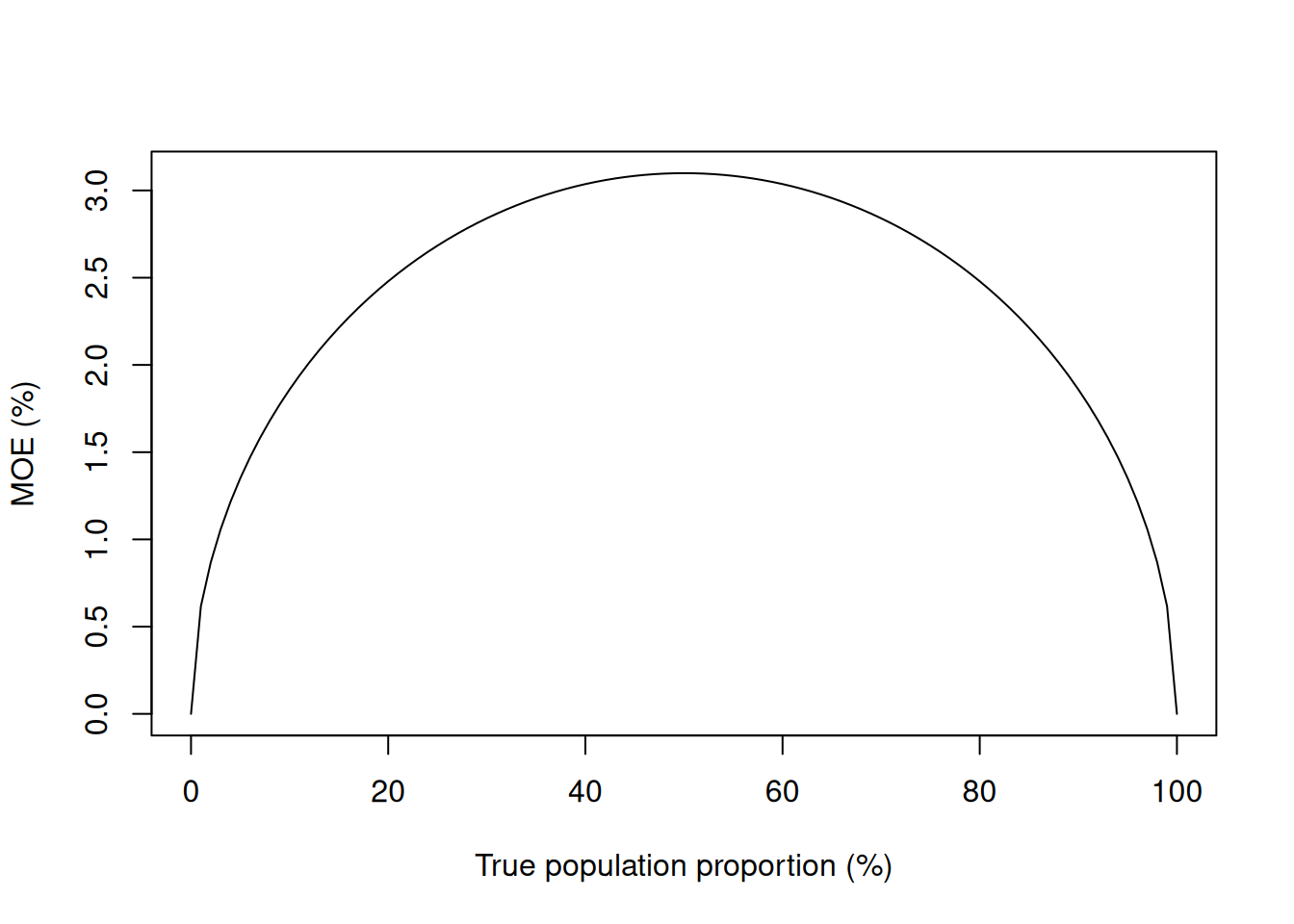
Figure 6.4: Dependence of the MOE for a proportion on the true population proportion (sample size n=1000).
While a party polling at 50% has an MOE of 3.2%, a party polling at 1% has a MOE of 0.62%, which is certainly not larger than 1%.
6.8 Derivation of sampling errors
In this section we give the derivations of the expressions in Section 6.4. We start with the probability distribution of the sample membership under SRSWOR.
6.8.1 Inclusion Probabilities
There are \(\binom{N}{n}\) samples in all. Of these, there are \(\binom{N-1}{n-1}\) samples which contain unit \(i\) and \(\binom{N-2}{n-2}\) samples which contain both units \(i\) and \(j\), \(i\neq j\). Since each sample has equal probability \(1/\binom{N}{n}\), the probability that unit \(i\) is included in the sample is: \[ \pi_{i} = \binom{N-1}{n-1}\left/ \binom{N}{n}\right. = \frac{n}{N} \qquad \text{for $i=1, \ldots , N$} \] This probability is called the 1st order inclusion probability.
The probability that both units \(i\) and \(j\) are included is: \[ \pi_{ij} = \binom{N-2}{n-2}\left/ \binom{N}{n}\right. = \frac{n\left(n-1\right)}{N\left(N-1\right)} \qquad \text{for $i,j=1, \ldots , N, i \neq j$} \] and this probability is called the joint inclusion probability or the 2nd order inclusion probability. Note that \(\pi_{ii}=\pi_i\).
Note: There are sampling schemes which have the same 1st and 2nd order inclusion probabilities equal to those from SRSWOR, but are not SRSWOR.
6.8.2 Sample Membership Indicator Variables
The sample membership indicator variable \(I_{i}\) is a random variable which takes the value one or zero for each unit \(i\) in the population. It is one if the unit is in the sample, and zero otherwise.
In a probability sampling scheme \(I_i\) is a random variable. Its mean value is just the 1st order inclusion probability: \[\begin{eqnarray*} \bfa{E}{I_i} &=& 0\times{\rm Pr}(I_i=0) + 1\times{\rm Pr}(I_i=1)\\ &=& 0\times(1-\pi_i) + 1\times\pi_i\\ &=& \pi_i \end{eqnarray*}\] Also note that \[\begin{eqnarray*} \bfa{E}{I_iI_j} &=& 0\times0\times{\rm Pr}(I_i=0,I_j=0) + 1\times0\times{\rm Pr}(I_i=1,I_j=0)\\ & & +\ 0\times1\times{\rm Pr}(I_i=0,I_j=1) + 1\times1\times{\rm Pr}(I_i=1,I_j=1)\\ &=& {\rm Pr}(I_i=1,I_j=1)\\ &=& \pi_{ij} \end{eqnarray*}\] so that the covariance of \(I_i\) and \(I_j\) is \[\begin{eqnarray*} \bfa{Cov}{I_i,I_j} &=& \bfa{E}{I_iI_j} - \bfa{E}{I_i}\bfa{E}{I_j}\\ &=& \left\{\begin{array}{ll} \pi_{ij}-\pi_i\pi_j\hspace{1ex}& \text{if $i\neq j$},\\ \pi_i(1-\pi_i) & \text{if $i=j$} \end{array} \right. \end{eqnarray*}\]
For simple random sampling and \(i\neq j\) we have \[\begin{eqnarray*} \pi_{ij} -\pi_i\pi_j &=& \left(\frac{n-1}{N-1}\right) \frac{n}{N} - \left(\frac{n}{N}\right)^2\\ &=& \frac{n}{N}\left[\frac{n-1}{N-1}-\frac{n}{N}\right]\\ &=& \frac{n}{N^2(N-1)}\left[(n-1)N-n(N-1)\right]\\ &=& \frac{n}{N^2(N-1)}(n-N)\\ &=& -\frac{n}{N(N-1)}\left(1-\frac{n}{N}\right) \end{eqnarray*}\] so that \[\begin{eqnarray*} \bfa{E}{I_i} &=& \frac{n}{N}\\ \bfa{Cov}{I_i,I_j} &=& \left\{\begin{array}{ll} -\frac{n}{N}\left(1-\frac{n}{N}\right)\frac{1}{N-1} \hspace{1ex}& \text{if $i\neq j$},\\ \frac{n}{N}\left(1-\frac{n}{N}\right) & \text{if $i=j$} \end{array} \right. \end{eqnarray*}\] In other words there is a (small) negative correlation between \(I_i\) and \(I_j\) for distinct units. If unit \(i\) is already selected it slightly decreases the chances that unit \(j\) will end up in the sample.
6.8.3 Horwitz-Thompson Estimator
One of the reasons for introducing the machinery of sample membership indicator random variables \(I_{i}\) and their expected values, is that it immediately gives us an estimator of the population total called the Horvitz-Thompson Estimator under any sampling scheme where the 1st order inclusion probabilities \(\pi_i\) are known and are non-zero. The HT estimator is \[\begin{eqnarray} \estm{Y}_{HT} &\equiv& \sum_{k\in s} \frac{y_{k}}{\pi_k}\\ \nonumber &=& \sum_{i\in U} I_i\frac{Y_i}{\pi_i} \end{eqnarray}\] (Here \(k\in s\) indicates the units in the sample, and \(i\in U\) the units in the population.)
We can show that the HT estimator is unbiased for \(Y\) by computing its mean: \[\begin{eqnarray*} \bfa{E}{\estm{Y}_{HT}} &=& \sum_{i\in U} \bfa{E}{I_i}\frac{Y_i}{\pi_i}\\ &=& \sum_{i\in U} \pi_i\frac{Y_i}{\pi_i}\\ &=& \sum_{i\in U} Y_i\\ &=& Y\\ \end{eqnarray*}\] Its variance follows straightforwardly too: \[\begin{eqnarray} \nonumber \bfa{Var}{\estm{Y}_{HT}} &=& \bfa{E}{Y_{HT}Y_{HT}} - \bfa{E}{Y_{HT}}\bfa{E}{Y_{HT}}\\ \nonumber &=& \sum_{i\in U} \sum_{j\in U} \bfa{E}{I_iI_j} \frac{Y_i}{\pi_i}\frac{Y_j}{\pi_j} - \sum_{i\in U} \sum_{j\in U} \bfa{E}{I_i}\bfa{E}{I_j} \frac{Y_i}{\pi_i}\frac{Y_j}{\pi_j}\\ \nonumber &=& \sum_{i\in U} \sum_{j\in U} \bfa{Cov}{I_i,I_j} \frac{Y_i}{\pi_i}\frac{Y_j}{\pi_j}\\ \nonumber &=& \sum_{i\in U} \frac{Y_i^2}{\pi_i^2}\bfa{Cov}{I_i,I_i} + \sum_{i\in U} \sum_{j\in U, j\neq i} \frac{Y_i}{\pi_i}\frac{Y_j}{\pi_j} \bfa{Cov}{I_i,I_j}\\ &=& \sum_{i\in U} \frac{Y_i^2}{\pi_i^2}\pi_i(1-\pi_i) + \sum_{i\in U} \sum_{j\in U, j\neq i} \frac{Y_i}{\pi_i}\frac{Y_j}{\pi_j} (\pi_{ij}-\pi_i\pi_j) \end{eqnarray}\] In the case of SRSWOR this variance becomes \[\begin{eqnarray} \nonumber \bfa{Var}{\estm{Y}_{HT}} &=& \sum_{i\in U} Y_i^2\frac{N^2}{n^2} \frac{n}{N}\left(1-\frac{n}{N}\right) - \sum_{i\in U} \sum_{j\in U, j\neq i} Y_iY_j\frac{N^2}{n^2} \frac{n}{N}\left(1-\frac{n}{N}\right)\frac{1}{N-1}\\ \nonumber &=& \frac{N}{n}\left(1-\frac{n}{N}\right)\frac{1}{N-1} \left[ (N-1) \sum_{i\in U} Y_i^2 - \sum_{i\in U} \sum_{j\in U, j\neq i} Y_iY_j \right]\\ \nonumber &=& \frac{N}{n}\left(1-\frac{n}{N}\right)\frac{1}{N-1} \left[ N \sum_{i\in U} Y_i^2 - \sum_{i\in U} \sum_{j\in U} Y_iY_j \right]\\ \nonumber &=& \frac{N^2}{n}\left(1-\frac{n}{N}\right) \frac{\sum_{i\in U} Y_i^2 - N\bar{Y}^2}{N-1}\\ &=& N^2\left(1-\frac{n}{N}\right) \frac{S_Y^2}{n} \end{eqnarray}\]
If we know the population size \(N\) then the estimator for the population mean \(\estm{\bar{Y}}_{HT}\) follows immediately from the estimator for the total: \[\begin{equation} \estm{\bar{Y}}_{HT} \equiv \frac{\estm{Y}_{HT}}{N} \end{equation}\] This estimator is unbiased for \(\bar{Y}\) since \[ \bfa{E}{\estm{\bar{Y}}_{HT}} = \frac{\bfa{E}{\estm{Y}_{HT}}}{N} = \frac{Y}{N} = \bar{Y} \] and its variance is \[\begin{eqnarray} \nonumber \bfa{Var}{\estm{\bar{Y}}_{HT}} &=& {\bf Var}\left[\frac{\estm{Y}_{HT}}{N}\right]\\ \nonumber &=& \frac{\bfa{Var}{\estm{Y}_{HT}}}{N^2}\\ &=& \left(1-\frac{n}{N}\right) \frac{S_Y^2}{n} \end{eqnarray}\]
6.9 Sampling errors in SRSWR
We can carry out a similar procedure to estimate the sampling error in the case of simple random sampling with replacement.
In this case the indicator variables \({\bf I}_{i=1}^N\) become the count of times that each unit is selected. In without replacement sampling \(I_i\) can only be 0 or 1, but in with replacement sampling \(I_i\) can take any value from 0 to \(n\), subject to their values adding to the total sample size \(n=\sum_{i=1}^N I_i\).
The full vector of \({\bf I}\) values follows a multinomial distribution: \[ {\bf I} \sim \text{Multinomial}(n,(1/N){\bf 1}) \] where each individual has a probability \(\frac{1}{N}\) of being selected on each of the \(n\) draws. Then: \[\begin{eqnarray*} \bfa{E}{I_i} &=& \frac{n}{N} = \pi_i\\ \bfa{E}{I_i^2} &=& \frac{n}{N}\left(1+\frac{n-1}{N}\right)\\ \bfa{E}{I_iI_j} &=& \frac{n(n-1)}{N^2} = \pi_{ij} \qquad \text{$i\neq j$} \end{eqnarray*}\] so that the covariance of \(I_i\) and \(I_j\) is \[\begin{eqnarray*} \bfa{Cov}{I_i,I_j} &=& \bfa{E}{I_iI_j} - \bfa{E}{I_i}\bfa{E}{I_j}\\ &=& \left\{\begin{array}{ll} -\frac{n}{N^2}& \text{if $i\neq j$},\\ \frac{n}{N}-\frac{n}{N^2} & \text{if $i=j$} \end{array} \right. \end{eqnarray*}\] As with SRSWOR there is a (small) negative correlation between \(I_i\) and \(I_j\) for distinct units. If unit \(i\) is already selected it slightly decreases the chances that unit \(j\) will end up in the sample.
We have the same unbiased HT estimator \[\begin{eqnarray} \estm{Y}_{HT} &\equiv& \sum_{k\in s} \frac{y_{k}}{\pi_k}\\ \nonumber &=& \sum_{i\in U} I_i\frac{Y_i}{\pi_i}\\ &=& \frac{N}{n} \sum_{i\in U} I_iY_i \end{eqnarray}\] with \[\begin{eqnarray*} \bfa{E}{\estm{Y}_{HT}} &=& \frac{N}{n} \sum_{i\in U} \bfa{E}{I_i}Y_i\\ &=& \frac{N}{n} \sum_{i\in U} \frac{n}{N} Y_i\\ &=& \sum_{i\in U} Y_i\\ &=& Y \end{eqnarray*}\]
In SRSWR the variance of this estimator is \[\begin{eqnarray*} \bfa{Var}{\estm{Y}_{HT}} &=& {\bf Var}\left[\frac{N}{n} \sum_{i\in U} I_iY_i\right]\\ &=& \frac{N^2}{n^2} \sum_{i\in U}\sum_{j\in U} {\bf Cov}\left[I_i,I_j\right] Y_iY_j\\ &=& \frac{N^2}{n^2} \sum_{i\in U}\sum_{j\in U} \left[-\frac{n}{N^2} + I(i=j)\frac{n}{N} \right] Y_iY_j\\ &=& -\frac{N^2}{n^2} \sum_{i\in U}\sum_{j\in U} \frac{n}{N^2}Y_iY_j + \frac{N^2}{n^2} \sum_{i\in U} \frac{n}{N} Y_i^2\\ &=& -\frac{1}{n}\sum_{i\in U}\sum_{j\in U} Y_iY_j + \frac{N}{n} \sum_{i\in U} Y_i^2\\ &=& -\frac{1}{n} N^2\bar{Y}^2 + \frac{N}{n} \left[(N-1)S_Y^2 + N\bar{Y}^2\right]\\ &=& N(N-1)\frac{S_Y^2}{n} \end{eqnarray*}\] (Here we’ve used the notation \(I(i=j)\), known as the indicator function, which is 1 if \(i=j\) and 0 if not.)
This is SRSWR variance very close to the SRSWOR variance \[\begin{eqnarray*} \bfa{Var}{\estm{Y}_{HT, SRSWOR}} &=& N^2\left(1-\frac{n}{N}\right)\frac{S_Y^2}{n} \end{eqnarray*}\] with the principal difference being the presence of the finite population correction factor \((1-\frac{n}{N})\) in the SRSWOR expression. In SRSWR even taking a sample of size \(n=N\) doesn’t guarantee a census, so there is still some sampling error left.