Chapter 4 Sampling and Estimation

\(\DeclareMathOperator*{\argmin}{argmin}\) \(\newcommand{\var}{\mathrm{Var}}\) \(\newcommand{\bfa}[2]{{\rm\bf #1}[#2]}\) \(\newcommand{\rma}[2]{{\rm #1}[#2]}\)

4.1 Sampling Error

Our aim is to estimate a population parameter \(T\), such as the unemployment rate, using a data from a sample of the population. In doing so we end up with an estimate \(\widehat{T}\) of \(T\), rather than the true value of \(T\) itself.

Setting all other sources of survey error aside for the moment, we will concentrate on sampling error: the error caused by taking a sample rather than doing a census. If we were to do a census, then we would simply be measuring the value of \(T\). Sampling error arises because the properties of a sample are (somewhat) different from the properties of the population from which the sample comes.

As an example, consider the small population of \(N=10\) people listed in Table 4.1, and the sizes of the families (total numbers of siblings) that they come from.

Table 4.1: Family size data

Person, \(i\)	Family Size, \(Y_i\)
1	3
2	5
3	1
4	4
5	9
6	3
7	2
8	4
9	6
10	2

The mean family size and total number of siblings in this population are \[ \bar{Y} = \frac{1}{N} \sum_{i=1}^N Y_i = 3.9 \ \ \ \text{and}\ \ \ Y = \sum_{i=1}^N Y_i = N\bar{Y} = 39 \] If I want to estimate \(\bar{Y}\), the mean family size, and I’m only allowed to take a sample of \(n=5\), I would draw five numbers at random between 1 and \(N=10\) (discarding duplicates) and then ask the five selected people how many siblings are in their families. I’d end up with five sample values \(\{y_1, y_2, y_3, y_4, y_5\}\) and would use mean of those values as an estimate of \(\bar{Y}\). For example if I draw random numbers \(\{8, 5, 2, 3, 1\}\) then the sample data are \[ \{y_1, y_2, y_3, y_4, y_5\} = \{Y_8, Y_5, Y_2, Y_3, Y_1\} = \{4, 9, 5, 1, 3\} \] with mean \(\bar{y}=4.4\), and standard deviation \(s_y=2.966\). I take the sample mean \(\bar{y}\) as my estimate \(\widehat{\bar{Y}}=\bar{y}=4.4\) of the true value \(\bar{Y}=3.9\).

Note: the sample mean \(\bar{y}=\frac{1}{n}\sum_k y_k\) is called the estimator of \(\bar{Y}\), and the value that comes from a particular sample, e.g. \(\bar{y}=4.4\), is called an estimate of \(\bar{Y}\). i.e. an estimator is a method of calculating an estimate.

Each sample will have different members, and a different mean. Thus the precision of the estimate \(\bar{y}\) from any given sample depends on how different samples can be from one another: i.e. the precision depends on the sampling variability.

Figure 4.1 shows a histogram displaying the distribution of family sizes of the 10 members of the population. These range from 1 to 9. The thick vertical line shows the population mean 3.9.

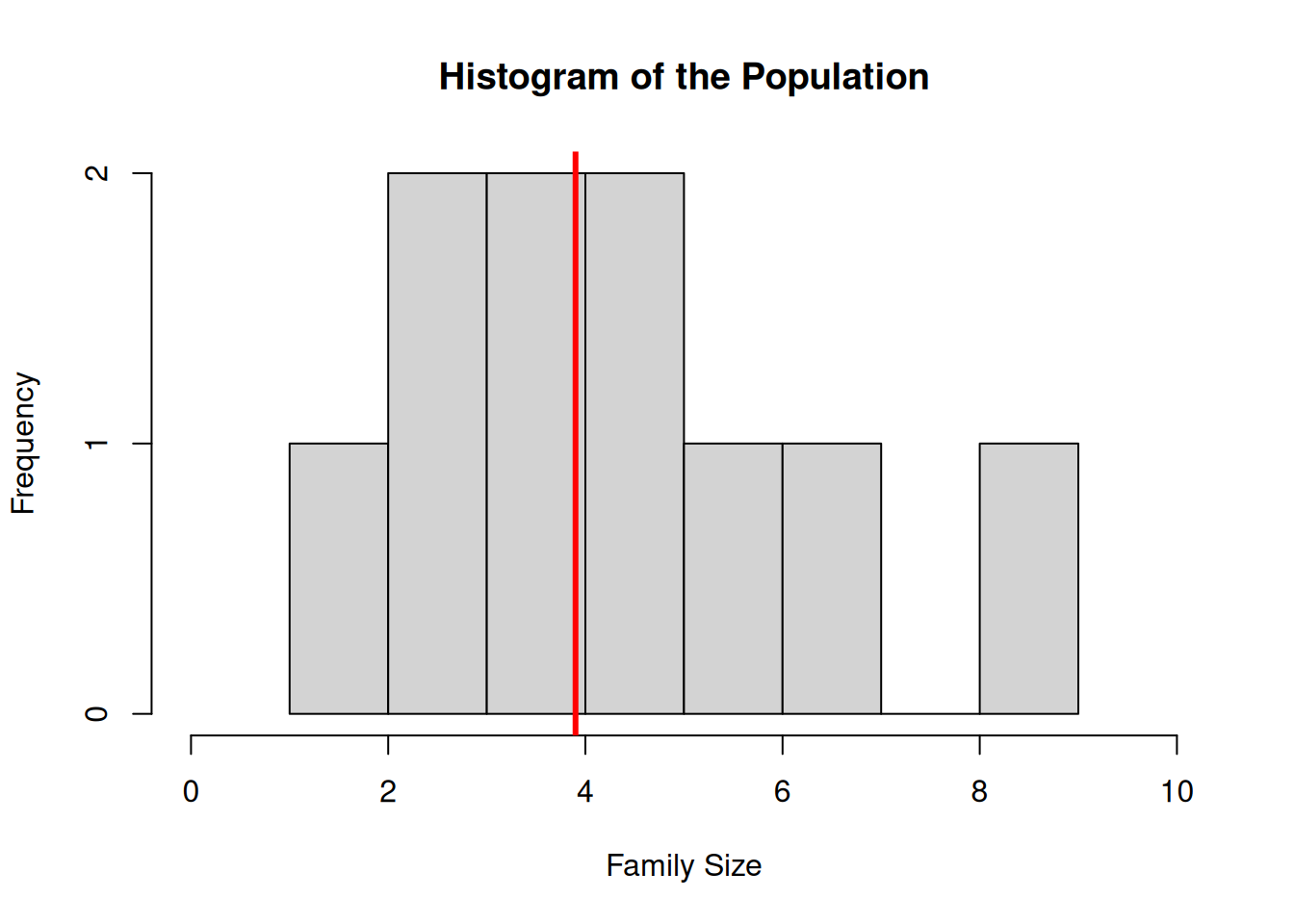
Figure 4.1: Histogram of Family sizes

The variance of the data in this histogram is the variance of the population: \[ S_Y^2 = \bfa{Var}{Y_i} = \frac{1}{N-1}\sum_{i=1}^N (Y_i-\bar{Y})^2 = 5.4333 = 2.33^2 \] The histogram in Figure 4.2 has been made by drawing from the population all of the 252 possible distinct samples of size 5, and then calculating the mean of each one.

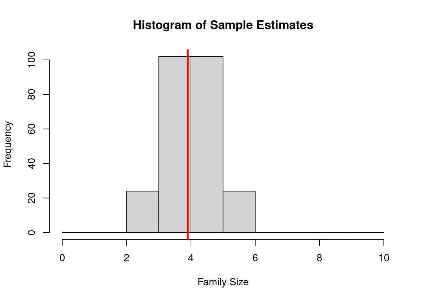
Figure 4.2: Histogram of estimates of mean family size in the 252 possible SRSWOR of size 5 drawn from the population

Note the following:

• The distribution of estimates from the 252 possible samples all cluster around the true mean 3.9;
• The distribution appears roughly normal (unimodal, symmetric, few/no outliers) – even though the data are not Normal;
• The variance of the distribution of sample means \(\bar{y}\) is less than the variance of the population: \[ \bfa{Var}{\bar{y}} = 0.545 = 0.739^2 \] The standard deviation of the \(\bar{y}\) values is called the standard error of the estimator \(\bar{y}\), and it can be used in standard ways to compute a confidence interval for \(\bar{Y}\). \[ \bfa{SE}{\bar{y}} = \sqrt{\bfa{Var}{\bar{y}}} = 0.739 \] This value comes from a consideration of all possible samples, and can only be calculated using full knowledge of all the population values.

However, based on our sample only, and ignoring the fact (that we’ll get to later) that this population is finite, we can approximate the standard error of our estimate of the mean using the sample standard deviation and sample size using the familiar formula: \[ \bfa{SE}{\bar{y}} = \frac{s_y}{\sqrt{n}} = \frac{2.966}{\sqrt{5}} = 1.326 \] So a 95% confidence interval for \(\mu\) based on our sample only is then \[\begin{eqnarray*} &&\bar{y} \pm 1.96\times \bfa{SE}{\bar{y}}\\ &&\bar{y} \pm 1.96\times \frac{\sigma}{\sqrt{n}}\\ &&\bar{y} \pm 1.96\times \frac{s_y}{\sqrt{n}}\\ &&4.4 \pm 1.96\times \frac{2.966}{\sqrt{5}}\\ &&4.4 \pm 1.96\times 1.326\\ &&4.4 \pm 2.6\\ &&(1.8, 7.0) \end{eqnarray*}\]

Note that the properties of samples vary less as the sample size gets bigger - see Figure 4.3, where we can see the sampling error decrease as \(n\) increases.
Ultimately when the sample size is \(n=N\), i.e. a census, there’s only one possible sample.

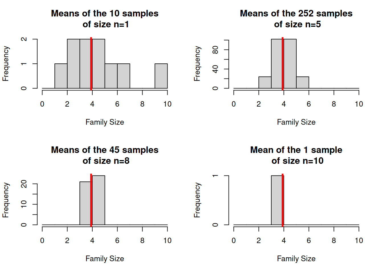
Figure 4.3: Histogram of estimates of mean family size in the possible SRSWOR of (a) size 1, (b) size 5, (c) size 8 and (d) size 10 drawn from the population

The diagram in Figure 4.4 is a picture of what is going on. We have a population of interest, which has a parameter or parameters that we want to estimate. We draw a sample according to some selection procedure, well aware that the properties of that sample will differ somewhat from those of the other possible samples that we might have drawn. Our inferences about the characteristics of the population must take this sampling variability into account. We can only make proper inferences about the population if we can assign a selection probability to all possible samples.

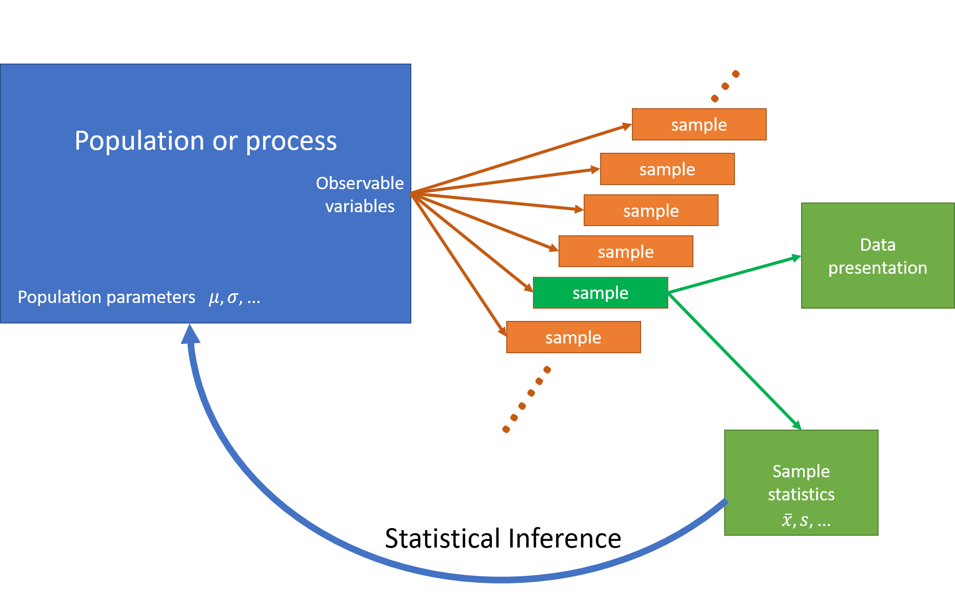
Figure 4.4: Statistical Inference. We draw a sample from the population, well aware that the properties of that sample will differ somewhat from those of the other possible samples that we might have drawn. Our inferences about the characteristics of the population must take this sampling variability into account.

4.2 Statistical Review

In earlier courses you will already have come across estimators of population parameters and their standard errors. A brief review of these estimators and their properties is given below. These formulae assume that the sampling is being done from infinite populations – however one of the important differences between the theory of sample surveys and the rest of statistics is the incorporation of the finite size of populations, and we will see important modifications to these formulae later.

• Estimation of a mean \(\mu\) from a sample of size \(n\) taken from a population with variance \(\sigma_y^2\):, \(\{y_1,\ldots,y_n\}\): \[ \widehat{\mu} = \bar{y} = \frac{1}{n}\sum_{k=1}^n y_k \] with standard error \[ \bfa{SE}{\widehat{\mu}} = \frac{\sigma_y}{\sqrt{n}} \simeq \frac{s_y}{\sqrt{n}} \] When the Central Limit Theorem holds the sampling distribution of \(\bar{y}\) is \[ \bar{y} \sim \text{Normal}\left(\mu,\frac{\sigma^2_y}{n}\right) \] and a large sample confidence interval is \[ \bar{y} \pm Z \times \frac{s_y}{\sqrt{n}} \]
• Estimation of a proportion \(p\) from a Binomial sample of size \(n\), where \(X\) = number of successes in \(n\) identical trials.
  \[ \widehat{p} = \frac{X}{n} \] with standard error \[ \bfa{SE}{\widehat{p}} = \sqrt{\frac{p(1-p)}{n}} \simeq \sqrt{\frac{\widehat{p}(1-\widehat{p})}{n}} \] When the Central Limit Theorem holds the sampling distribution of \(\widehat{p}\) is \[ \widehat{p} \sim \text{Normal}\left(p,\sqrt{\frac{p(1-p)}{n}}\right) \] and a large sample confidence interval is \[ \widehat{p} \pm Z \times \sqrt{\frac{\widehat{p}(1-\widehat{p})}{n}} \]

The large sample results rely on the Central Limit Theorem, and \(Z=1.96\) for 95% confidence. A confidence interval is always stated as: \[ \begin{split} &\text{estimate} \pm \text{margin of error}\\ &\widehat{T} \pm \bfa{MOE}{\widehat{T}}\\ &\widehat{T} \pm Z\times\sqrt{\bfa{Var}{\widehat{T}}}\\ &\widehat{T} \pm Z\times\bfa{SE}{\widehat{T}} \end{split} \] Also note that a proportion is in fact just a special case of a mean. If on \(n\) Binomial trials we record \(y_k=1\) for a success and \(y_k=0\) for a failure, (i.e. \(y_k\) is an indicator variable) then the proportion of successes is \[ \widehat{p} = \frac{1}{n} \sum_{k=1}^n y_k = \frac{1 + 0 + 1 + 0 + 0 + 1 + 0 + 0 + \ldots}{n} = \frac{X}{n} \] For this reason we do not have to treat means and proportions separately: one is just a special case of the other.

4.3 Expected Value, Bias and Mean Squared Error

Given a population the choice of a sample design defines a set of all possible samples: this set is called the sample space, \(\mathbb{S}\), which may be enormous. (In the example above, a random sample of 5 people from a population of size 10 means that there are 252 possible samples). In any given survey we measure just one of the elements of the sample space \(s\), and we can calculate the probability of obtaining that sample \(p(s)\).

An estimator \(\widehat{T}(s)\) of a population parameter \(T\) (e.g. the total or mean of a variable \(Y\)) is a random variable. Under a probabilistic sampling scheme it takes on a different value for every sample \(s\) that can be drawn under that scheme.

The mean (expected) value of an estimator \(\widehat{T}(s)\) is given by \[ \bfa{E}{\widehat{T}} = \sum_{s\in{\mathbb{S}}} p(s) \widehat{T}(s) \] and its variance is \[ \bfa{Var}{\widehat{T}} = \sum_{s\in{\mathbb{S}}} p(s) \left(\widehat{T}(s)-\bfa{E}{\widehat{T}}\right)^2 \] The variance is a strong indicator of the quality of the estimator. The standard error is the square root of the variance: \[ \bfa{SE}{\widehat{T}} = \sqrt{\bfa{Var}{\widehat{T}}} \]

The sampling bias of an estimator is defined to be the difference between the mean value of the estimator, and the population parameter: \[ \bfa{Bias}{\widehat{T}} = \bfa{E}{\widehat{T}}-T \] (Note that the sampling bias excludes any biases due to non-sampling error - such as non-response, questionnaire bias, respondent error etc.)

The diagram in Figure 4.5 shows the situation: the error of an estimator is a combination of bias and variance.

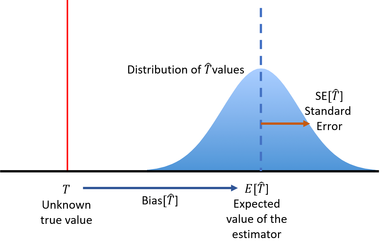
Figure 4.5: An estimator \(\widehat{T}\) of a population parameter \(T\) has a sampling distribution with a mean \(\bfa{E}{\widehat{T}}\), standard error \(\bfa{Var}{\widehat{T}}\), variance \(\bfa{Var}{\widehat{T}}=\bfa{Var}{\widehat{T}}^2\), and possible bias \(\bfa{Bias}{\widehat{T}}\).

Where an estimator is biased, we use the mean squared error as a measure of quality, instead of the variance: \[ \bfa{MSE}{\widehat{T}} = \bfa{E}{(\widehat{T}-T)^2} = \bfa{Var}{\widehat{T}} + \bfa{Bias}{\widehat{T}}^2 \] The MSE combines the effects sampling variance and sampling bias together. A low variance estimator may be highly biased, and we may instead prefer an estimator with a higher variance but with lesser bias (Figure 4.6).

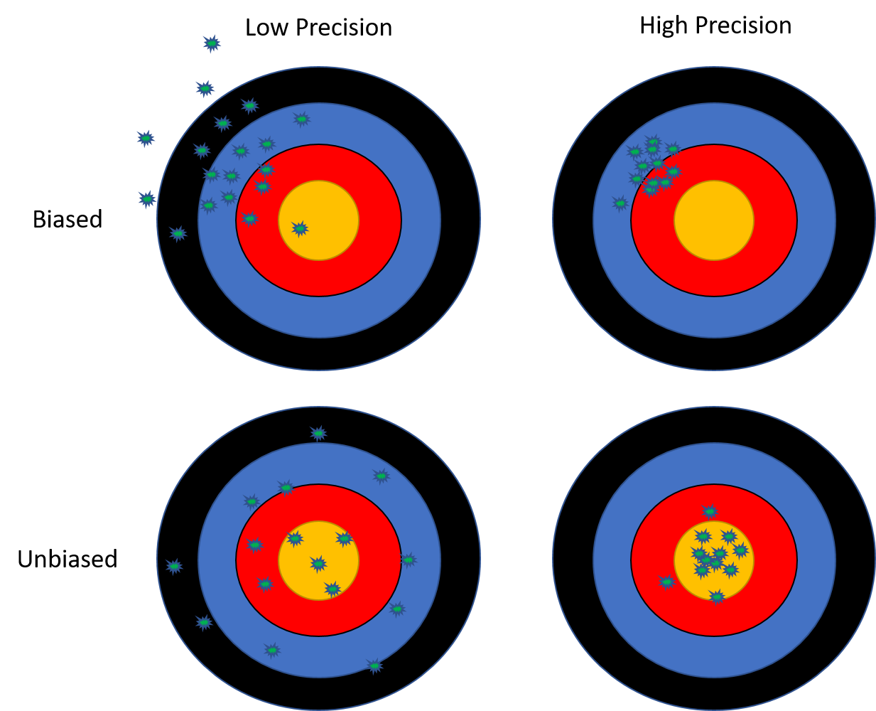
Figure 4.6: In general we prefer zero bias and low variance estimators. A low variance but highly biased estimate is usually unacceptable,and we may have to put up with high variance in order to eliminate bias. However a small bias is acceptable if this reduces the variance significantly.

4.3.1 Example

Under simple random sampling, the sample mean \(\bar{y}\) is an unbiased estimator \(\widehat{\mu}\) of the population mean \(\mu\): \[\begin{eqnarray*} \bfa{E}{\widehat{\mu}} &=& \mu\\ \bfa{Var}{\widehat{\mu}} &=& \frac{\sigma^2}{n}\\ \bfa{Bias}{\widehat{\mu}} &=& \bfa{E}{\widehat{\mu}}-\mu=\mu-\mu=0\\ \bfa{MSE}{\widehat{\mu}} &=& \bfa{Var}{\widehat{\mu}}+\bfa{Bias}{\widehat{\mu}}^2 = \frac{\sigma^2}{n} + 0 = \frac{\sigma^2}{n} \end{eqnarray*}\] We will come across estimators which are biased later in the course (e.g. the ratio estimator is an example of a biased estimator).

4.4 What are the advantages of sampling?

• reduced cost;
• quicker to carry out resulting in improved timeliness;
• greater scope - sampling can allow for greater scope and flexibility due to it being less resource demanding. Often specialised personnel are scarce meaning that a complete census is impracticable;
• improved accuracy and quality - often the time saved due to sampling can be put into more intensive and careful collection and checking of the data. More specialised training of the survey personnel is possible, allowing for an improved control of non-sampling error;
• reduced burden on respondents.

4.5 What are the disadvantages of sampling?

• sampling error;
• less scope for detailed analysis of the data: may not obtain sufficient data for analysis of specific sub-populations;
• technical knowledge required by survey staff (e.g. random selection of participants);
• Public perception – small groups may worry that they are not adequately represented in the results if a sample rather than a census is taken.

4.6 Approaches to sampling

• Probability Sampling. Every sample in the sample space has a known chance of selection, and it follows that every member of the population also has a known nonzero probability of selection. These properties allow the probability distribution and other properties of estimators to be derived.
• Purposive or Judgement Sampling. The surveyor chooses a sample which they believe, based on their knowledge of the population, to be ‘representative’. Alternatively the sample is chosen to cover the diversity present in the population.
• Quota Sampling. Sample sizes or quotas are set for different types of unit in the population (e.g. age/sex groups). Units are selected until these quotas are met.
• Haphazard Sample. Use whatever sample is available. e.g. ‘People I know.’ Snowball samples (where sample members recruit other sample members).
• Self-selected Sample. Volunteers phoning in, or writing letters.

Non-probability samples are entirely legitimate if a survey is qualitative. For example, a survey may aim to sample the full range of views held by all members of a population, in order to generate hypotheses which can be tested in a quantitative survey. A purposive sample is used to scatter the sample widely, rather than attempting to select a representative sample. Pilot surveys often have non-probability samples.

A purposive step in an otherwise probabilistic design may be acceptable: e.g. a random sample of people from Wellington may be justifiably thought to be similar on certain characteristics (e.g. reaction to using certain drugs) to people elsewhere. For practical reasons the survey can be justifiably restricted to Wellington, but the results can be generalised to the whole country. The justification for the generalisation needs to be sound, and can remain open to question.

4.7 Examples of sampling schemes

4.7.1 SRSWOR=Simple Random Sample WithOut Replacement.

Here we want to estimate the average number of hours spent by students majoring in Science on coursework at VUW.

We obtain a list of all students majoring in Science from the Registry. We assign a number from 1 to \(N\), the total number of such students, to each student. We select \(n\) distinct random numbers between 1 and \(N\) from a set of random number tables. If the random number \(i\) is chosen then we select the \(i\)th student. Then we collect the necessary information from the student.

4.7.2 STSRS=Stratified Simple Random Sample.

We might want to estimate the number of employees in food retailers. We have a list of \(N\) businesses to select from, and the earnings of each retailer in the past year.

We classify the retailers into several groups (called strata) based on their earnings: there \(H\) strata, with \(N_h\) retailers in group \(h\) (for \(h=1,\ldots,H\)). We take a SRSWOR of \(n_h\) retailers from each stratum, and count the number of employees in each sampled retailer.

4.7.3 LSRS=Linear Systematic Random Sample.

Here we want to estimate the proportion of visitors to New Zealand who intend to stay for more than 2 weeks. Visitors can be selected at the airport as they pass through customs. We choose a time to start sampling, and then select at random one passenger in the first twenty. Thereafter we sample every twentieth arriving passenger.

4.7.4 SRS1C=One-stage Cluster Sample.

Here we want to estimate the number of shellfish categorized by species, e.g. pipis, mussels, etc on a beach.

At low tide we divide the beach into 1m \(\times\) 1m quadrats. We number each quadrat, from 1 to \(N\). We select \(n\) distinct random numbers between 1 and \(N\) from a set of random number tables. If the random number \(i\) is chosen then we select the \(i\)th quadrat. We dig up the quadrat and count the number of shellfish.

4.7.5 SRS2C=Two-stage Cluster Sample.

Again we want to estimate the number of shellfish.

This is a big beach, e.g. Titahi Bay. So at low tide we divide the beach into 10m \(\times\) 10m quadrats. We number each quadrat, from 1 to \(N\). We select \(n\) distinct random numbers between 1 and \(N\) from a set of random number tables. If the random number \(i\) is chosen then we select the \(i\)th quadrat – this is the first stage of sampling. Now for each selected quadrat we further divide the quadrat into one hundred 1m \(\times\) 1m (sub)quadrats. We number these from 1 to 100. We select \(m\) distinct random numbers between 1 and 100 from a set of random number tables. If the random number \(j\) is chosen then we select the \(j\)th (sub)quadrat, within the \(i\)th quadrat – this is the second stage of sampling. We dig up the (sub)quadrat and count the number of shellfish.

4.7.6 STSRS1C=Stratified Cluster Sample.

Again we want to estimate shellfish, but now just mussels. The beach has some sandy strips and some rocky outcrops, and mussels are more likely to be found on the rocky outcrops.

We split the beach into areas which are either predominantly sandy, or predominantly rocky. At low tide within each of these areas, \(h\), we divide the beach into 1m \(\times\) 1m quadrats. We number each quadrat, from 1 to \(N_{h}\). We select \(n_{h}\) distinct random numbers between 1 and \(N_{h}\) from a set of random number tables. If the random number \(i\) is chosen then we select the \(i\)th quadrat. Note that, each of the samples in the different areas of the beach are independent. We dig up the quadrat and count the number of shellfish.

4.7.7 PPSWR=Selection Probability Proportional to Size, With Replacement.

We want to estimate the number of calves born in spring on farms supplying milk for Town Milk Supply. We have information on the number of milking cows on each such farm and indeed each cow is registered on a computer database. Suppose the cows are labelled 1 to \(N\). We select \(n\) random numbers between 1 and \(N\) from a set of random number tables. If the random number \(i\) is chosen and the \(i\)th cow belongs to farm \(j\), then we select farm \(j\) and ask them to tell us how many calves were born.

4.8 Adminstrative Data - a common alternative to sampling

Administrative Data are data which are collected during the routine operations of an organisation as it manages its client population. Examples include

• Hospital admissions
• GP Prescriptions
• Student records in a University
• Tax records
• Aircraft movements at an airport

Such data sets can help us understand the population of interest, and importantly:

• They are complete - the entire managed population is represented;
• They are often of high quality - since the data they contain are necessary to the management of the population;
• They are up to date, containing all activities in the population right up to the current moment;
• The data already exist, so are a cheap form of data collection, provided we can get permission to gain access;
• The sample sizes can be very large.

These characteristics make admin data sets excellent sources of information about a population.

However, they have some distinct drawbacks:

• Available administrative data sets may not exactly match our target population.

  e.g. we may be interested in the health of all New Zealanders, whereas the hospital admissions data set only covers people with severe conditions which require hospitalisation, and they only cover public hospitals.

• They are transactional - the fundamental unit of the data may be an interaction (e.g. an episode of hospital care) rather than a member of the population. This can make them complicated to analyse: some people may appear multiple times in the data set, and others not at all. We also need to be able to match people properly so we can identify which records refer to the same individual;

• They only contain information relevant to the operation of the organisation that collects the data - the things we may want to know aren’t available.

  e.g. although we may find out what operations a person had in hospital, we can’t know who they felt about it. For our analyses we may also want to know information about a person’s income or education - things that aren’t collected by the health system because they’re not needed to manage care;

• We can see the most recent interaction of a person with the organisation - but we can’t know if that person is still alive now, or is still in the country, so we don’t know if they are part of our population anymore.

• The definitions used to define data items may differ from ones we want to use, or may change over time.

  e.g. Diagnostic codes regularly undergo revision, which means when comparing older with newer data we may have to use different sets of codes in different time periods. We may be interested in the rate of occurrence of complications up to one year after surgery, but the data may only record complications up to 30 days.

The power of administrative data sets can be enhanced by linkage: individuals in a number of data sets can be identified and their records linked, as a way of increasing the richness of the information available for analysis. Statistics New Zealand’s Integrated Data Infrastructure (IDI) is an example of a data linkage warehouse where many data sets (census, tax, health, eduction etc) are linked, enabling more powerful analyses.

While administrative data may be suitable to answer many questions, some can really only be answered by a sample survey.