Chapter 12 Regression Estimation

\(\DeclareMathOperator*{\argmin}{argmin}\) \(\newcommand{\var}{\mathrm{Var}}\) \(\newcommand{\bfa}[2]{{\rm\bf #1}[#2]}\) \(\newcommand{\rma}[2]{{\rm #1}[#2]}\) \(\newcommand{\estm}{\widehat}\)

Regression models are everywhere in statistics, and when we are working with sample survey data we are not always only interested in population level estimates, but also the relationships between variables in the data.

12.1 Regression models with survey data

In regression we assume a relationship between one variable – the outcome, \(Y\) – and a set of explanatory variables – the predictors, \(X\).

For example if we have just one predictor variable then the simple linear regression model is
\[\begin{equation} Y_i = \alpha + \beta X_i + \varepsilon_i \qquad \text{for $i=1,\ldots,N$} \tag{12.1} \end{equation}\] Here \(\alpha\) and \(\beta\) are the familiar intercept and slope of a linear regression problem with one variable. The errors \(\varepsilon_i\) are assumed to be independent and identically distributed, with a Normal distribution with mean 0 and variance \(\sigma^2\).

The focus of our interest is usually on the value of \(\beta\) – which quantifies the relationship (if any exists) between \(X\) and \(Y\).

Fitting regression models in sample survey models is possible, but does require some care thought: we need to be aware that the data may not necessarily be a simple random sample, and that the data may have unequal weights.

Some software packages can accept weights in regression, but one must be very careful to recognise that the word ‘weight’ can mean one of three different things.

1. Frequency Weights – the weight is the number of times the observation appears in the dataset – this is a compact way of representing data where there are many repetitions. An observation has high weight if it has been seen multiple times;
2. Precision Weights – when there is measurement error, an observation has high precision weight if it is measured very precisely, lower weight if it was measured imprecisely;
3. Sampling Weights – these are our survey sampling weights: the inverse of the probability of selection. An observation has high weight if it had a low probability of selection, and represents a large number of units in the population.

Statistical software that allows weights may be a bit vague in the documentation about what the weights mean. It’s imperative to be sure that you know which type of weights the software is using.

Through the specification of sample designs, iNZight treats sample weights correctly, and we can be confident about the results that it produces. The Advanced Modelling window allows the fitting of a variety of regression models, and returns parameter estimates, standard errors and confidence intervals allowing us to use survey data to investigate relationships.

There is some discussion about whether or not sampling weights actually need to be included in regression analyses, even with survey data. However the consensus is that it (almost) never harms your analysis to include the weights, and there are times when it can save you from biased estimates.

12.2 Regression estimation

We came across the idea of regression imputation in our analysis of non-response. We fitted a relationship between \(X\) and \(Y\) for the observed data, and imputed values for \(Y\) where they were missing using the predicted values from the regression model: \[ \widehat{y}_k = \widehat{\alpha} + \widehat{\beta} x_k \] We could do this within the sample when we had either measured values of \(x_k\) for all of the respondents (including the ones where \(y_k\) was missing).

This suggests a more general approach to survey sampling estimation. We can regard all of the population members that we didn’t select as non-respondents, and use a regression method to impute their unobserved \(Y\) values. Then we can make estimates of the population mean and total of \(Y\) using those imputed values.

This is a very powerful idea.

Consider the set of \(N=16\) NZ regions and their volumes of retail trade in 2019, listed in Table 12.1 and also plotted in Figure 12.1.

Table 12.1: Retail trade volumes and populations in NZ regions in 2019

	Region	Volume ($M)	Population	Population (000)
1	Northland	827.2	188700	188.7
2	Auckland	10146.2	1642800	1642.8
3	Waikato	2445.5	482100	482.1
4	Bay of Plenty	1714.3	324200	324.2
5	Gisborne	201.8	49300	49.3
6	Hawke’s Bay	829.8	173700	173.7
7	Taranaki	549.6	122700	122.7
8	Manawatu-Wanganui	1150.7	249700	249.7
9	Wellington	2578.3	527800	527.8
10	Tasman	250.3	54800	54.8
11	Nelson	320.1	52900	52.9
12	Marlborough	256.4	49200	49.2
13	West Coast	180.6	32600	32.6
14	Canterbury	3409.7	628600	628.6
15	Otago	1470.3	236200	236.2
16	Southland	543.8	101200	101.2

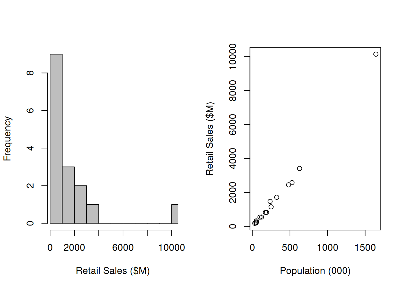
Figure 12.1: Retail trade volumes and populations in NZ regions in 2019

It’s very clear, and also logical, that population and volume of retail trade are correlated with one another. And it’s also clear that if we took a random sample of regions and happened to miss out Auckland that we’d severely underestimate the amount of retail trade.

The true total is \(Y=2.68746\times 10^{4}\), and the the standard deviation across the 16 regions is \(S_Y=2459.8\) (both in millions of dollars).

If we were to take a SRSWOR of \(n=6\) regions then the standard error of an estimate of the population total retail trade derived from a sample of size \(n=6\) would be \[\begin{eqnarray*} \bfa{SE}{\widehat{Y}} &=& \sqrt{N^2\left(1-\frac{n}{N}\right)\frac{S_Y^2}{n}}\\ &=& \sqrt{(16)^2\left(1-\frac{6}{16}\right)\frac{2459.8^2}{6}}\\ &=& 1.27023\times 10^{4} \end{eqnarray*}\] which would give an RSE of \[\begin{eqnarray*} \bfa{RSE}{\widehat{Y}} &=& \frac{\bfa{SE}{\widehat{Y}}}{Y}\\ &=& \frac{1.27023\times 10^{4}}{2.68746\times 10^{4}}\\ &=& 0.47 \end{eqnarray*}\] An appallingly bad 47%.

If we take an actual sample of \(n=6\) observations (Table 12.2) then our sample statistics are \(n=6\), \(\bar{y}=691.8\) and \(s_y=543.1\).

Table 12.2: Retail trade volumes and populations in NZ regions in 2019: SRS of 6 regions

		Region	Volume ($M)	Population	Population (000)
1	1	Northland	827.2	188700	188.7
5	5	Gisborne	201.8	49300	49.3
8	8	Manawatu-Wanganui	1150.7	249700	249.7
11	11	Nelson	320.1	52900	52.9
13	13	West Coast	180.6	32600	32.6
15	15	Otago	1470.3	236200	236.2

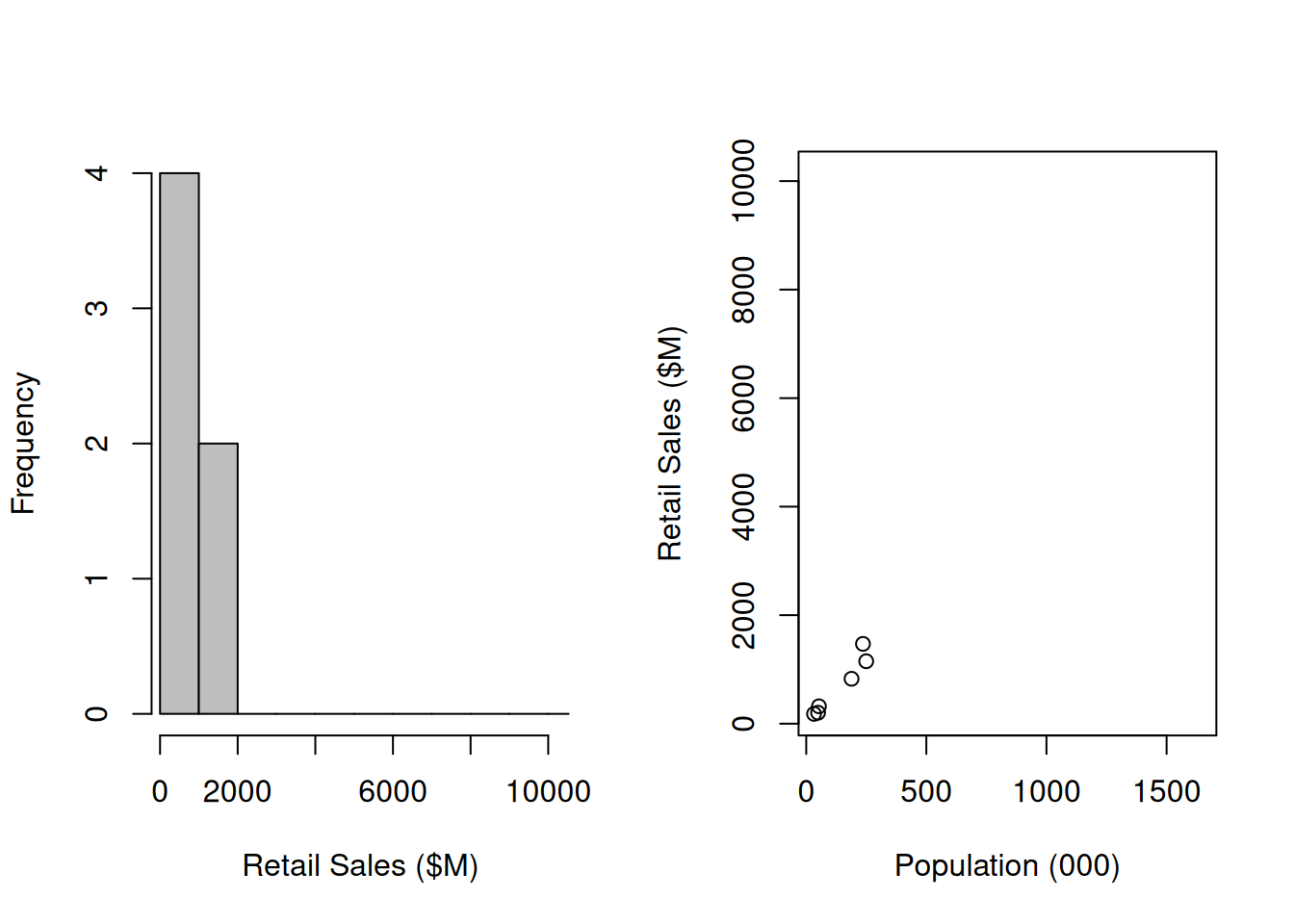
Figure 12.2: Sample of retail trade volumes and populations in NZ regions in 2019

This leads to an estimate of the total national volume of \[ \widehat{Y} = N\bar{y} = (16)(691.8) = 1.1069\times 10^{4} \] which – due to Auckland not being in the sample – is dramatically less than the truth (\(2.6875\times 10^{4}\)), and has standard error \[\begin{eqnarray*} \bfa{SE}{\widehat{Y}} &=& \sqrt{N^2\left(1-\frac{n}{N}\right)\frac{s_y^2}{n}}\\ &=& \sqrt{(16)^2\left(1-\frac{6}{`16}\right)\frac{543.1^2}{6}}\\ &=& 2804 \end{eqnarray*}\] This standard error is also underestimated (again, due to the absence of Auckland), and we have a false sense of security. The estimated RSE (\(2804/(1.1069\times 10^{4})=0.25\)) is still very bad though (primarily due to the small sample size).

Regression estimation is a way to protect us in situations like this. If the value of the population \(X_i\) is known for all regions, but we only have data on retail trade volumes \(Y_i\) for a sample of regions, then we can fit a regression relationship between \(Y\) and \(X\) in the sample. A sensible model is not the usual linear regression model but instead a no-intercept model: \[ Y_i = \beta X_i + \varepsilon_i \] in which retail trade \(Y_i\) is proportional to regional population size \(X_i\).

Fitting this model using iNZight, or a similar package that incorporates survey sample designs, we obtain estimates of \(\beta\) and its standard error: \[ \widehat{\beta} = 5.145448 \qquad \bfa{SE}{\widehat{\beta}} = 0.401191 \] We can use this fitted model to predict the value of \(Y_i\) for all of the unobserved regions.
\[ \widehat{Y}_i = \widehat{\beta} X_i \] For example, we estimate the retail trade in Auckland (\(i=2\), population \(X_2=1642.8\) thousand people) as \[ \widehat{Y}_2 = \widehat{\beta} X_2 = (5.145448)(1642.8) = 8452.9 \] this estimate has standard error \[ \bfa{SE}{\widehat{Y}_2} = \bfa{SE}{\widehat{\beta}X_2} = \bfa{SE}{\widehat{\beta}} X_2 = (0.401191)(1642.8) = 659 \]

All of the true data \(Y_i\) (of which we have only sampled 6 points) and the estimated data \(\widehat{Y}_i\) are plotted in Figure 12.3.
The model does a great job at estimating retail trade volumes using the population.

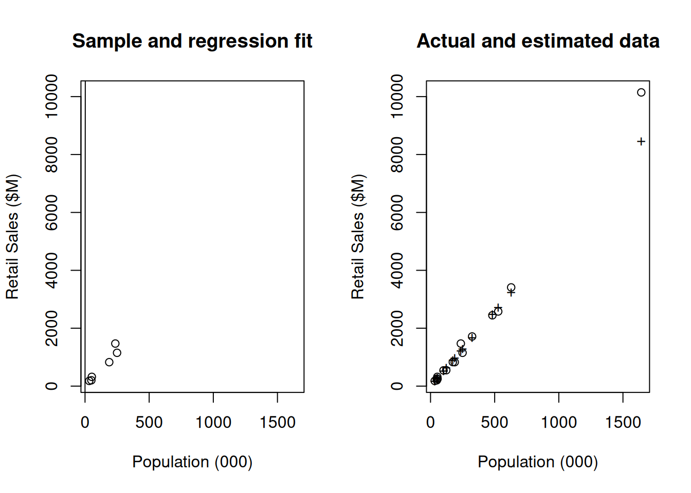
Figure 12.3: Regression estimation: at left is the sample and the fitted regression model. At right we have used the model to predict all of the data (+ symbols), and have plotted the true data (open circles) for comparison

We can make an estimate of the total retail trade over all regions using these estimated volumes: \[\begin{eqnarray*} \widehat{Y} &=& \sum_{i=1}^N \widehat{Y}_i\\ &=& \sum_{i=1}^N \widehat{\beta} X_i\\ &=& \widehat{\beta} \sum_{i=1}^N X_i\\ &=& \widehat{\beta} X \end{eqnarray*}\] where \(X=\sum_{i=1}^N X_i=4916.5\) is the total population (in thousands) of all regions combined. Thus \[ \widehat{Y} = (5.145448)(4916.5) = 2.5298\times 10^{4} \] which is now much much closer to the true value of \(2.68746\times 10^{4}\). The standard error of the estimate is \[ \bfa{SE}{\widehat{Y}} = \bfa{SE}{\widehat{\beta}} X = (0.401191)(4916.5) = 1972 \] which has an RSE of \(1972/(2.5298\times 10^{4})=0.078=7.8\)% – this result is a reduction from an apparent RSE of 25% to 7.8% is a dramatic improvement in the quality of our estimate – which is still from a very small sample.

12.3 More complex regression models

We can generalise this simple example by using a whole set of auxiliary variables \(X^{(1)}_i, X^{(2)}_i, X^{(3)}_i, \ldots\) and modelling the dependence of the outcome \(Y_i\) as either a linear regression problem: \[\begin{eqnarray}\nonumber Y_i &=& \beta_0 + \beta_1 X^{(1)}_i + \beta_2 X^{(2)}_i + \beta_3 X^{(3)}_i + \ldots + \varepsilon_i\\ \tag{12.2} &=& \beta_0 + \sum_{j=1}^q \beta_j X^{(j)} + \varepsilon_i \end{eqnarray}\] or still further if we allow \(Y\) to depend on the set of auxiliary variables in some more complex form \[\begin{equation} Y_i = f(X^{(1)}_i, X^{(2)}_i, \ldots; \theta) + \varepsilon_i \end{equation}\] where \(f()\) is a function with a form which we choose, and \(\theta\) are parameters that are to be estimated.

The most common regression model used is the linear model (Equation (12.2)). We set up the model with the \(q\) variables of interest. For example in the case of the modelling military expenditure in a set of countries we might include GDP and population as sensible predictor variables. In which case our model would be \[ Y_i = \beta_0 + \beta_1 \text{(population)}_i + \beta_2 \text{(GDP)}_i \] which in matrix notation can be written \({\bf Y}=X\boldsymbol{\beta}\).

Software such as iNZight (and more particularly the R survey package which iNZight uses) can be used for all of the familiar regression models that you will have seen in other settings. What is important though, is that the sample design must be appropriately incorporated. If the sample design is not included in the analysis we’ll end up with biased estimates, incorrect standard errors, and erroneous conclusions.

12.4 Ratio estimation

In the standard no-intercept regression model we assume that \[ Y_i = \beta X_i + \varepsilon_i \qquad\text{with}\qquad \varepsilon_i\overset{\rm iid}{\sim}N(0,\sigma^2) \] That is, the variance of the errors is constant \(\sigma^2\).

If we assume that all the units are independent, but that the variance of each individual \(Y_i\) value is \(\sigma_i^2=\sigma^2X_i\) then we have the slightly different model \[ Y_i = \beta X_i + \varepsilon_i \qquad\text{with}\qquad \varepsilon_i\overset{\rm ind}{\sim}N(0,\sigma^2X_i) \] In this model the variance of the errors is \(\sigma^2 X_i\): i.e. it grows with \(X_i\). Thus where \(X\) is a larger there is a larger scatter of \(Y\) around the model.

The best estimate of \(\beta\) in this model is \[\begin{eqnarray*} \widehat{{\beta}}_R &=& \frac{\sum_k y_k}{\sum_k x_k}\\ &=& \frac{\bar{y}}{\bar{x}} \end{eqnarray*}\] This is the what is known as the classical ratio estimator \(\widehat{\beta}_R\). This estimator is very close to the constant variance estimator, but its variance is slightly different: \[ \bfa{Var}{\widehat{\beta}_R} = \frac{1}{\bar{x}^2}\left(1-\frac{n}{N}\right)\frac{s_e^2}{n} \] where \(s_e^2\) is the variance of the residuals \[ s_e^2 = \frac{1}{n-1}\sum_{k=1}^n (y_k-\widehat{y}_k)^2 \] and \(\bar{x}\) is the sample mean. It leads to a familiar looking variance estimator for the population mean: \[ \bfa{Var}{\widehat{\bar{Y}}_R} = \left(1-\frac{n}{N}\right)\frac{s_e^2}{n} \] the difference being that the sample variance \(s_y^2\) is replaced by the residual variance \(s_e^2\).

Continuing the retail trade example above: we have the sample mean of retail trade being \(\bar{y}=691.8\) and the sample mean of the population \(\bar{x}=135\) (in thousands of people).

First estimate \(\beta\): \[ \widehat{\beta}_R = \frac{\bar{y}}{\bar{x}} = \frac{691.8}{135} = 5.12812 \] Next compute the fitted values \(y_k=\widehat{\beta}_Rx_k\) and the residuals \[\begin{eqnarray*} e_k &=& \text{Observed} - \text{Calculated}\\ &=& y_k - \widehat{y}_k\\ &=& y_k - \widehat{\beta}x_k \end{eqnarray*}\] For example: \[\begin{eqnarray*} \widehat{y}_1 &=& \widehat{\beta}_Rx_1\\ &=& (5.12812)(188.7)\\ &=& 967.7\\ e_1 &=& y_1 - \widehat{y}_1\\ &=& 827.2 - 967.7\\ &=& -140.5 \end{eqnarray*}\]

All of the fitted values \(\widehat{y}_k\) and the residuals \(e_k\) are shown in Table 12.3. The standard deviation of the residuals is \(s_e=147.53\).

Table 12.3: Sample with fitted values and residuals

Area, \(i\)	Region	Volume, \(y_k\)	Population (000), \(x_k\)	Fitted Volumes, \(\widehat{y}_k\)	Residuals, \(e_k=y_k-\widehat{y}_k\)
1	Northland	827.2	188.7	967.7	-140.5
5	Gisborne	201.8	49.3	252.8	-51.0
8	Manawatu-Wanganui	1150.7	249.7	1280.5	-129.8
11	Nelson	320.1	52.9	271.3	48.8
13	West Coast	180.6	32.6	167.2	13.4
15	Otago	1470.3	236.2	1211.3	259.0

The variance of the population mean is then \[\begin{eqnarray*} \bfa{Var}{\widehat{\bar{Y}}_R} &=& \left(1-\frac{n}{N}\right)\frac{s_e^2}{n}\\ &=& \left(1-\frac{6}{16}\right)\frac{147.53^2}{6}\\ &=& 2267.32 = (47.62)^2 \end{eqnarray*}\] The variance of the ratio estimate of \(\beta\) is (noting again that the mean size of the 6 sampled regions is \(\bar{x}=135\)): \[\begin{eqnarray*} \bfa{Var}{\widehat{\beta}_R} &=& \frac{1}{\bar{x}^2}\left(1-\frac{n}{N}\right)\frac{s_e^2}{n}\\ &=& \frac{1}{(135)^2}\left(1-\frac{6}{16}\right)\frac{147.53^2}{6}\\ &=& 0.1245916 = (0.352975)^2 \end{eqnarray*}\]

Our interest is in the total retail trade volume: \[\begin{eqnarray*} \widehat{Y} &=& N\widehat{\bar{Y}}\\ &=& N\widehat{\beta}_R\bar{X}\\ &=& \widehat{\beta}_R X \end{eqnarray*}\] where \(X\) is the total population \(X=4916.5\): \[\begin{eqnarray*} \widehat{Y} &=& (5.12812)(4916.5) = 2.5212\times 10^{4} \end{eqnarray*}\] (almost identical to our earlier regression estimate of \(2.5298\times 10^{4}\)).

The standard error of this estimate is \[ \bfa{SE}{\widehat{Y}} = \bfa{SE}{\widehat{\beta}_RX} = \bfa{SE}{\widehat{\beta}_R}X = (0.352975)(4916.5) = 1735.4 \] This is reduced from our regression SE of \(1972\) with RSE \(1735.4/2.52124\times 10^{4} = 0.069\) – and is a better estimate of our uncertainty due to the fact that the variance of retail trade really does increase with \(X\).