Chapter 2 The Basics
2.1 Loading a dataset
iNZight works with one dataset at a time. The first thing to do is load up a dataset.
- Example data: iNZight comes with a number of built-in data sets. The ones from the
surveypackage are most relevant to us. To load one into iNZight go:File > Example Data- Set the
Module (package)to beSurvey - Choose a
Dataset– for exampleapisrs (api)is a dataset of academic performance of a sample of 200 schools from California.
- Click
OK
- Read a dataset from a file: iNZight needs there to be a top row of column names, and then the data
- Go
File > Import Data - Browse for the data set you want (supported options include
.csv,.txtand.xlsx) - Click
Import
- Go
2.2 Viewing a dataset
There are two data view buttons at the top left:
View Data Setshows the data set contents - good for getting an idea of what is in your dataset.View Variablesgives a list of the variables (the titles of the columns) - this is the best view for the analyses to follow. In this view iNZight labels each variable as(c)(Categorical) or(n)(Numerical).
You can remove (‘filter out’) rows using Dataset > Filter - specifying a condition to be applied to a specific variable. This creates a new dataset for you to work with. You can switch between datasets with the Data set: window drop-down menu at upper left (under the View Data Set/View Variables buttons).
2.3 Transform variables
Various conversions/transformations are possible using options under the Variables menu.
Of particular interest are:
- Change the numerical variables to categorical (
Variables > Convert to Categoricalthen choose the variable you want to convert, choose a new name for it, thenUpdate) - Delete one or more variables from the dataset (
Variables > Delete Variables) - Rename variables
- Create new variables, by computing them from the values in other columns
After you’ve made changes to a dataset, you can export it to save your work: File > Export Data.
2.4 Overall properties of the data
With no variables in the slots Variable 1-Variable 4 at lower left, click Get Summary right at bottom left. You’ll see characteristic of each variable, including variable ranges (numerical variables), numbers of distinct values (categorical variables), and numbers of missing observations.
2.4.1 Example
In the apisrs dataset Get Summary shows:
====================================================================================================
                                   iNZight summary of "apisrs_ex"
----------------------------------------------------------------------------------------------------
   Number of observations (rows): 200
   Number of variables (columns): 39 (28 numeric and 11 categorical)

====================================================================================================
Numeric variables:
------------------

                  min       max   n. missing
       snum     59.00   6157.00            0
       dnum      1.00    832.00            0
       cnum      1.00     56.00            0
       flag       Inf      -Inf          200
    pcttest     83.00    100.00            0
      api00    348.00    965.00            0
      api99    347.00    952.00            0
     target      1.00     23.00           19
     growth    -22.00    189.00            0
      meals      0.00    100.00            0
        ell      0.00     89.00            0
   mobility      0.00     67.00            0
     acs.k3     15.00     30.00           60
     acs.46     14.00     37.00           42
   acs.core     17.00     34.00          140
   pct.resp      0.00    100.00            0
    not.hsg      0.00     84.00            0
        hsg      0.00     75.00            0
   some.col      0.00    100.00            0
   col.grad      0.00     59.00            0
   grad.sch      0.00     67.00            0
     avg.ed      1.18      4.67            7
       full     26.00    100.00            1
       emer      0.00     78.00            1
     enroll    131.00   2106.00            0
    api.stu    111.00   1717.00            0
         pw     30.97     30.97            0
        fpc   6194.00   6194.00            0


Categorical variables:
----------------------

              n. categories   n. missing
        cds               0            0
      stype               3            0
       name               0            0
      sname               0            0
      dname               0            0
      cname               0            0
   sch.wide               2            0
   comp.imp               2            0
       both               2            0
     awards               2            0
     yr.rnd               2          180

====================================================================================================
2.5 Simple estimates
2.5.1 Numerical Variables
With a numerical variable are often interested in means and standard deviations of the data:
- in
View Variablesview, drag a numerical variable onto theVariable 1window at lower left. A graph immediately appears at right, displaying the distribution of the variable as a combined dot-plot and box-plot. - You can save this or any graph in iNZight by clicking the save icon (just to the left of the X icon at the bottom of the screen). (Note - the right-click+Save option directly on the graph doesn’t work, at least not for me.)
- Click
Get Summmary
2.5.1.1 Example
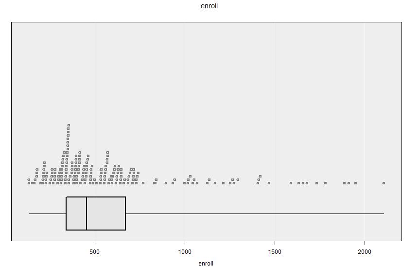
apisrs dataset. The data are right skewed (having a long tail to the right: i.e. to large values): there are many small schools of similar sizes, and just a few larger schools with widely differing sizes.Output of Get Summary:
====================================================================================================
                                          iNZight Summary
----------------------------------------------------------------------------------------------------
   Primary variable of interest: enroll (numeric)

   Total number of observations: 200
====================================================================================================

Summary of enroll:
------------------

Population estimates:

   Min   25%   Median     75%    Max    Mean      SD   Sample Size
   131   339      453   668.5   2106   584.6   393.5           200


====================================================================================================
2.5.1.2 Inference
For inference we are interested in an estimate of the population mean, its standard error, and a 95% confidence interval.
- Leaving everything as above, click
Get Inference- leave the defaults as they are
This gives an estimate of the population mean, along with the lower and upper bounds of a 95% confidence inverval.
2.5.1.3 Example
Inference for the Enrolment size enroll variable in the apisrs dataset:
====================================================================================================
                               iNZight Inference using Normal Theory
----------------------------------------------------------------------------------------------------
   Primary variable of interest: enroll (numeric)

   Total number of observations: 200
====================================================================================================

Inference of enroll:
--------------------

Mean with 95% Confidence Interval

   Lower    Mean   Upper
   529.7   584.6   639.5


====================================================================================================
2.5.2 Categorical variables
With a categorical variable are want to know the counts and proportions in each category:
- in
View Variablesview, drag a categorical variable onto theVariable 1window at lower left. A graph immediately appears at right, displaying the distribution of the variable as a barchart. - Click
Get Summmary
2.5.2.1 Example
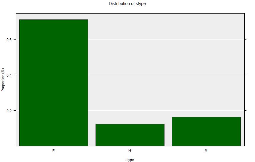
stype in the apisrs dataset. The schools of type ‘E’ are small Elementary (Primary) schools - and there are many of these. There are many fewer, and larger middle schools (‘M’) and High Schools (‘H’).====================================================================================================
iNZight Summary
----------------------------------------------------------------------------------------------------
Primary variable of interest: stype (categorical)
Total number of observations: 200
====================================================================================================
Summary of the distribution of stype:
-------------------------------------
E H M Total
Count 142 25 33 200
Percent 71.00% 12.50% 16.50% 100%
====================================================================================================2.5.2.2 Inference
For inference we are interested in an estimate of the population proportion, its standard error, and a 95% confidence interval.
- Leaving everything as above, click
Get Inference- leave the defaults as they are
This gives an estimate of the proportion in each category, along with the lower and upper bounds of a 95% confidence inverval for each category. The inference procedure creates estimates of the pairwise differences between the proportions in the various categories, also with 95% confidence intervals for these differences.
2.5.2.3 Example
Inference for the School Type stype variable in the apisrs dataset
====================================================================================================
                               iNZight Inference using Normal Theory
----------------------------------------------------------------------------------------------------
   Primary variable of interest: stype (categorical)

   Total number of observations: 200
====================================================================================================

Inference of the distribution of stype:
---------------------------------------

Estimated Proportions with 95% Confidence Interval

        Lower   Estimate   Upper
   E   0.6471      0.710   0.773
   H   0.0792      0.125   0.171
   M   0.1136      0.165   0.216


## Differences in proportions of stype
    (col group - row group)

Estimates

           E       H
   H   0.585
   M   0.545   -0.04

95% Confidence Intervals

            E          H
   H   0.4662
       0.7038
   M   0.4163   -0.13091
       0.6737    0.05091


====================================================================================================
2.6 Two-variable analyses
We are rarely interested in just one variable, more commonly we are interested in the existence (if any) and nature of the association between two variables. There are three broad cases to consider: two numerical variables, one numerical and one categorical, or two categorical variables.
2.6.1 Two numerical variables
This is simple regression.
- Drag two numerical variables into the
Variable 1andVariable 2positions - A scatter plot will be displayed
Get Summarywill show the Spearman’s rank correlation coefficient of the two variablesGet Inferencewill show the output of a linear regression - withVariable 1as the dependent (outcome) variable, andVariable 2as the independent (predictor) variable. Choose aLinear Trendfor a simple linear fit, though you can fit up to a cubic polynomial. This will also add the fitted relationship onto the diagram.
2.6.1.1 Example
In the apisrs dataset api00 is the year 2000 academic performance of each School, and meals is the percentage of students receiving school meals. Use api00 as Variable 1 and meals as Variable 2.
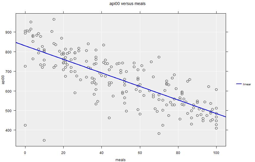
api00 against meals, showing linear regression fit. The greater the proportion of the student body receiving school meals, then lower the overall academic performance of the school.Summary output:
====================================================================================================
                                          iNZight Summary
----------------------------------------------------------------------------------------------------
        Response/outcome variable: api00 (numeric)
   Predictor/explanatory variable: meals (numeric)

     Total number of observations: 200
====================================================================================================

Summary of api00 versus meals:
------------------------------

Rank correlation: -0.79  (using Spearman's Rank Correlation)


====================================================================================================
Inference output:
====================================================================================================
                               iNZight Inference using Normal Theory
----------------------------------------------------------------------------------------------------
        Response/outcome variable: api00 (numeric)
   Predictor/explanatory variable: meals (numeric)

     Total number of observations: 200
====================================================================================================

Inference of api00 versus meals:
--------------------------------


Linear Trend Coefficients with 95% Confidence Intervals

               Estimate    Lower     Upper   p-value
   Intercept     829.37   806.75    851.99    <2e-16
       meals     -3.455   -3.843   -3.0669    <2e-16


   p-values for the null hypothesis of no association, H0: beta = 0


====================================================================================================
There is a clear negative relationship between proportion of children receiving school meals (a marker of socioeconomic deprivation) and academic performance.
2.6.2 One numerical and one categorical variable
This is Analysis of Variance (ANOVA).
- Drag the numerical variable into the
Variable 1position, and the categorical variable onto theVariable 2position - Parallel dot-plot/box-plots of the numerical variable will be shown for each level of the categorical variable
Get Summarywill show numerical summaries of the numerical variable within each category (mean, std deviation etc.)Get Inference(selectingANOVA) will show the output of an ANOVA - withVariable 1as the dependent (outcome) variable, andVariable 2as the independent (predictor) variable.
2.6.2.1 Example
In the apisrs dataset api00 is the year 2000 academic performance of each School, and stype is the type of school (Elementary, Middle or High). Use api00 as Variable 1 and stype as Variable 2.
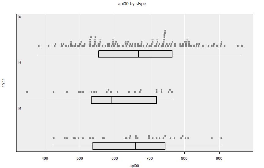
api00 against stype. There is no apparent relationship between school type and academic performance.Summary output:
====================================================================================================
                                          iNZight Summary
----------------------------------------------------------------------------------------------------
   Primary variable of interest: api00 (numeric)
             Secondary variable: stype (categorical)

   Total number of observations: 200
====================================================================================================

Summary of api00 by stype:
--------------------------

Population estimates:

       Min     25%   Median     75%   Max    Mean      SD   Sample Size
   E   382   553.5      668   764.2   965   666.1   135.7           142
   H   348   533.0      590   720.0   764   605.4   113.5            25
   M   425   537.0      660   744.0   905   654.3   129.1            33


====================================================================================================
Inference output:
====================================================================================================
                               iNZight Inference using Normal Theory
----------------------------------------------------------------------------------------------------
   Primary variable of interest: api00 (numeric)
             Secondary variable: stype (categorical)

   Total number of observations: 200
====================================================================================================

Inference of api00 by stype:
----------------------------

Group Means with 95% Confidence Intervals

       Lower    Mean   Upper
   E   643.6   666.1   688.7
   H   558.5   605.4   652.2
   M   608.5   654.3   700.1

One-way Analysis of Variance (ANOVA F-test)

   F = 2.2547, df = 2 and 197, p-value = 0.10761

          Null Hypothesis: true group means are all equal
   Alternative Hypothesis: true group means are not all equal


### Difference in mean api00 between stype groups
    (col group - row group)

Estimates

           E        H
   H   60.78
   M   11.87   -48.91

95% Confidence Intervals (adjusted for multiple comparisons)

             E         H
   H    -6.904
       128.470
   M   -48.439   -131.66
        72.175     33.83

P-values

           E      H
   H   0.088
   M   0.888   0.34


====================================================================================================
No convincing association between school type and academic performance.
2.6.3 Two categorical variables
This leads to a contingency table and a Chi-square test of association.
- Drag the two categorical variables into the
Variable 1andVariable 2positions - Grouped bar charts of the two variables will display
Get Summarywillshow a contingency table of counts and proportions (within rows) withVariable 1as the row variable andVariable 2is the column variable (swap them if it is more interpretable the other way around)Get Inference(selectingChi-square test) will show the row proportions and 95% confidence intervals for the contingency table. It will also show the result of a Chi-square test for association, and (within each level ofVariable 2) the pairwise differences in the proportions among the categories ofVariable 1(with 95% confidence intervals).
2.6.3.1 Example
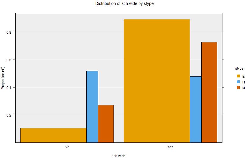
In the apisrs dataset sch.wide is a binary (Yes/No) variable indicating whether or not the School met its growth goals, and stype is the type of school (Elementary, Middle or High). Use sch.wide as Variable 1 and stype as Variable 2.
 Summary output:
====================================================================================================
                                          iNZight Summary
----------------------------------------------------------------------------------------------------
   Primary variable of interest: sch.wide (categorical)
             Secondary variable: stype (categorical)

   Total number of observations: 200
====================================================================================================

Summary of the distribution of sch.wide (columns) by stype (rows):
------------------------------------------------------------------

Table of Counts:

       No   Yes   Row Total
   E   15   127         142
   H   13    12          25
   M    9    24          33

Table of Percentages:

          No     Yes   Total   Row N
   E   10.6%   89.4%    100%     142
   H     52%     48%    100%      25
   M   27.3%   72.7%    100%      33


====================================================================================================
Inference output:
====================================================================================================
                               iNZight Inference using Normal Theory
----------------------------------------------------------------------------------------------------
   Primary variable of interest: sch.wide (categorical)
             Secondary variable: stype (categorical)

   Total number of observations: 200
====================================================================================================

Inference of the distribution of sch.wide (columns) by stype (rows):
--------------------------------------------------------------------

Estimated Proportions

          No     Yes   Row sums
   E   0.106   0.894          1
   H   0.520   0.480          1
   M   0.273   0.727          1

95% Confidence Intervals

           No     Yes
   E   0.0551   0.844
       0.1562   0.945
   H   0.3242   0.284
       0.7158   0.676
   M   0.1208   0.575
       0.4247   0.879

Chi-square test for equal distributions

   X^2 = 26.225, df = 2, p-value = 2.02e-06
   Simulated p-value (since some expected counts < 5) = 0.00049975

          Null Hypothesis: distribution of sch.wide does not depend on stype
   Alternative Hypothesis: distribution of sch.wide changes with stype


### Differences in proportions of stype with the specified sch.wide

  # Group differences between proportions with: sch.wide = No
    (col group - row group)

Estimates

            E         H
   H   0.4144
   M   0.1671   -0.2473

95%  Confidence Intervals

             E           H
   H   0.21210
       0.61663
   M   0.00695   -0.495153
       0.32724    0.000607

  # Group differences between proportions with: sch.wide = Yes
    (col group - row group)

Estimates

             E        H
   H   -0.4144
   M   -0.1671   0.2473

95%  Confidence Intervals

              E           H
   H   -0.61663
       -0.21210
   M   -0.32724   -0.000607
       -0.00695    0.495153


====================================================================================================
There is a clear relationship between school type and achievement of school wide growth goals: with High schools much less likely to achieve their growth goals.