Chapter 5 Cluster Sampling
In cluster sampling the population is first divided into \(N\) groups, known as clusters of Primary Sampling Units (PSUs), and a random sample of \(n\) clusters is selected. In one-stage cluster samples a census is taken of all units in each selected sample. In two-stage cluster samples a simple random sample of \(m_k\) units is taken from the \(M_k\) units in \(k^{\mathrm{th}}\) selected cluster.
5.1 One-Stage Cluster Sampling
In order for iNZight to carry out an appropriate analysis of a one-stage cluster design, we need to tell iNZight how many clusters there are in the population, and identify which units in the sample come from which cluster. We don’t need to specify the cluster sizes \(M_k\), since a census is taken of each selected cluster and thus iNZight can work out how big the clusters are. In iNZight this means
- adding a column to the dataset with the label \(k\) of the cluster to which each sample unit belongs, and then
- adding a column to the dataset with \(N\): the total number of clusters in the population
- telling iNZight that the data should be treated as a one-stage cluster sampling, and specifying the columns with the cluster labels and number of clusters.
We’ll assume that the two extra columns are already in the data set under consideration.
To tell iNZight to use these columns:
Dataset > Survey Design > Specify Design- In the
1st stage clustering variablebox choose the name of the cluster label variable - In the
Finite population correctionbox choose the name of the variable containing the number of clusters \(N\) - Click
OK
The probability of selection of the \(k^{\mathrm{th}}\) cluster in the sample is \[ \pi_k = \frac{n}{M} \] In a one-stage cluster sample all units in each selected cluster are selected, so the probability of selection of a sample unit is the same as the probability that the cluster is selected. So the probability that unit \(\ell\) in cluster \(k\) is selected is \[ \pi_{k\ell} = \frac{n}{M} \] So the survey weights are the same for all selected units \[ w_{k\ell} = \frac{N}{n} \]
5.1.1 Example
apiclus1 is a one-stage cluster sample of schools in California. The clusters are School Districts (stored in the variable dnum), and the variable fpc contains the value 757: the number \(N\) of School Districts. In the sample \(n=15\) districts are chosen, and then all of the schools (the units) are selected from those districts. A total of \(m=183\) schools were chosen in the 15 clusters.
To tell iNZight that this is one-stage cluster sample drawn from \(N=757\) districts, specify dnum as the 1st stage clustering variable, andfpc` as the Finite population correction.
Look at school size (Variable 1 = enroll) and school type (Variable 2 = stype).
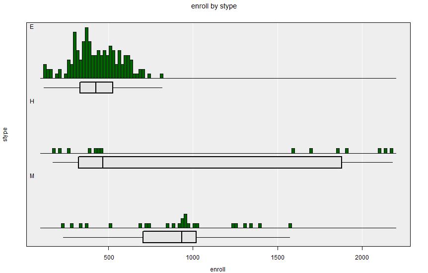 The Elementary Schools are smallest, and dominate the sample. The Middle and High Schools have a wide range of sizes.
Summary output:
====================================================================================================
                                  iNZight Summary - Survey Design
----------------------------------------------------------------------------------------------------
   Primary variable of interest: enroll (numeric)
             Secondary variable: stype (categorical)

   Total number of observations: 183
      Estimated population size: 9235
----------------------------------------------------------------------------------------------------
   1 - level Cluster Sampling design
   With (15) clusters.
   survey::svydesign(id = ~ dnum, fpc = ~ fpc, data = dataSet)
====================================================================================================

Summary of enroll by stype:
---------------------------

Population estimates:

          25%   Median       75%       Mean       SD        Total   Est. Pop. Size   |   Sample Size   Min    Max
   E   332.00   425.00    527.00    432.854   141.11   3145637.80           7267.2   |           144   117    818
   H   323.00   467.00   1881.50   1130.286   843.10    798584.53            706.5   |            14   170   2181
   M   704.00   935.00   1021.00    897.720   355.20   1132623.40           1261.7   |            25   233   1573

Standard error of estimates:

   E    17.33    23.78     36.68     16.516    16.69    941356.77           1988.0
   H   326.13   425.23    378.74    357.122    52.24    338039.77            236.6
   M   158.23    95.37    148.87     99.532    54.31    318535.53            249.8

Design effects:

   E                                  2.013                123.80
   H                                  2.563                  4.60
   M                                  2.003                 12.89

====================================================================================================
Note here that we estimate that there are \(Y_1=3.14\) million students in an estimated \(\widehat{M}_1=7267\) elementary schools, with a mean school size of \(\widehat{\bar{Y}_1}=433\) students.
5.2 Two-stage Cluster sampling
In a two-stage cluster sample we draw \(n\) clusters from the \(N\) in the population by SRS. Then we draw \(m_k\) units from the \(M_k\) units in the \(k^{\mathrm{th}}\) selected cluster.
In order for iNZight to carry out an appropriate analysis of a one-stage cluster design, we need to tell iNZight how many clusters there are in the population, and identify which units in the sample come from which cluster. We also need to specify the cluster sizes \(M_k\), since a only a sample of \(m_k\) units is taken of each selected cluster and thus iNZight needs to know how big the clusters are. In iNZight this means
- adding a column to the dataset with the label \(k\) of the cluster to which each sample unit belongs, and then
- adding a column to the dataset with \(N\): the total number of clusters in the population
- adding a column to the dataset with \(M_k\): the total number of units in the \(k^{\mathrm{th}}\) cluster from which the unit is taken
- telling iNZight that the data should be treated as a two-stage cluster sampling, and specifying the columns with the cluster labels, total number of clusters, and cluster sizes.
We’ll assume that the three extra columns are already in the data set under consideration.
To tell iNZight to use these columns:
Dataset > Survey Design > Specify Design- In the
1st stage clustering variablebox choose the name of the cluster label variable - In the
2nd stage clustering variablebox choose the name of the variable labelling individual units - In the
Finite population correctionbox choose the name of the column with the number of clusters \(M\) - In the
Finite population correction (2nd stage)choose the name of the column with the number of units per cluster \(N_k\).
- Click
OK
[Note: older versions of iNZight for Windows only have one Finite population correction box:
in that case type var1+var2 into the box, where var1 is the name of the population sizes
of the first stage \(M\) and var2 is the name of the population sizes at the second stage
\(N_k\).]
The probability of selection of the \(k^{\mathrm{th}}\) cluster in the sample is \[ \pi_k = \frac{n}{N} \] In a two-stage cluster sample we select by SRS \(m_k\) of the \(M_k\) units in each selected cluster, so the probability of selection of a sample unit is the product of two SRS selection probabilities: the probability that unit \(\ell\) in cluster \(k\) is selected is \[ \pi_{k\ell} = \frac{n}{N}\times\frac{m_k}{M_k} \] So the survey weights are the same for all selected units in the same cluster, but differ between clusters: \[ w_{k\ell} = \frac{NM_k}{nm_k} \]
5.2.1 Example
apiclus2 is a two-stage cluster sample of schools in California. The clusters are School Districts (stored in the variable dnum), the variable snum identifies the Schools within clusters. The variable fpc1 contains the value 757: the number \(M\) of School Districts, and fpc2 gives \(M_k\), the number of schools in the cluster from which each school was selected. In the sample \(n=40\) districts are chosen, and then a sample of between 1 and 5 schools was taken by SRS from each selected cluster. A total of 126 schools were selected.
To tell iNZight that this is two-stage cluster sample drawn from \(N=757\) districts:
- specify
dnumas the1st stage clustering variable - specify
snumas the2nd stage clustering variable, - type
fpc1+fpc2as the Finite population correction - to indicate the two population size columns (In the online version of iNZight putfpc1in the Finite population correction field, andfpc2in the 2nd finite population correction field.)
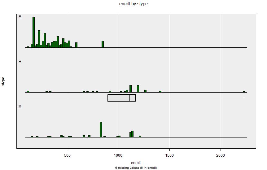
As before, look at school size (Variable 1 = enroll) and school type (Variable 2 = stype).
(Note iNZight may become significantly slow to run when specifying a complex design like this.)
Summary output:
====================================================================================================
                                  iNZight Summary - Survey Design
----------------------------------------------------------------------------------------------------
        Primary variable of interest: enroll (numeric)
                  Secondary variable: stype (categorical)

        Total number of observations: 126
   Number omitted due to missingness: 6 (6 in enroll)
   Total number of observations used: 120
           Estimated population size: 5129
----------------------------------------------------------------------------------------------------
   2 - level Cluster Sampling design
   With (40, 126) clusters.
   survey::svydesign(id = ~ dnum + snum, fpc = ~ fpc1+fpc2, data = dataSet)
====================================================================================================

Summary of enroll by stype:
---------------------------

Population estimates:

          25%    Median       75%        Mean       SD        Total   Est. Pop. Size   |   Sample Size   Min    Max
   E   219.75    295.60    437.43    339.7874   159.80   1161343.98           3493.6   |            83   113    840
   H   899.14   1114.75   1171.04   1038.6374   390.70    715486.12            688.9   |            20   112   2237
   M   720.00    800.92   1061.68    839.3250   279.00    762442.83            946.3   |            23   156   1211

Standard error of estimates:

   E    27.59     78.82    121.24     51.0810    28.88    334451.85           1119.7
   H   232.01    184.75     51.12     81.5152    97.21    338720.99            289.4
   M   149.18     78.66    105.74     67.5015    49.05    291735.04            311.8

Design effects:

   E                                   8.2586                 30.31
   H                                   0.8966                 32.62
   M                                   1.2529                 28.36
====================================================================================================
5.2.2 Supplying Weights
As in the one-stage design we are free to specify weights rather than supplying the details of the PSUs - in that case we still need to specify the 1st stage clustering variable (cluster labels, \(k\)) and the Finite population correction (Number of clusters, \(N\)), but after that we can supply a weighting variable in place of the individual label and the cluster size (\(M_k\)) values.