Chapter 3 Simple Random Sampling
In a simple random sample without replacement (SRSWOR) of size \(n\) from a population of size \(N\), every possible combination of \(n\) distinct population members has an equal chance of selection. This also means that the probability that any individual population member is selected is \(\pi=n/N\), and the weight each sample member carries in inference is \(w=N/n\).
3.1 Drawing a SRSWOR
If we have a dataset loaded we can use iNZight to select a SRSWOR from it:
- Go
Dataset > Filter > randomlythenProceed - Specify the
Sample Size\(n\) (must be less than or equal to the number of rows in the dataset), and only ask for 1 sample. - iNZight creates a new dataset with
.filteredadded to the end of the dataset name
You can choose a single sample of \(n\) rows, or multiple samples of \(n\) rows. If you choose more than one sample then iNZight creates a single dataset, but adds a final column Sample.Number which indicates which sample each row belongs to. If you ask for \(m=10\) samples of \(n=50\) rows then you will have a filtered dataset that is 500 lines long. Each set of 50 rows is a new sample, and note that although all of the members within an individual sample are distinct, it is possible for an individual to appear in more than one sample.
3.2 Properties of a SRSWOR
The number of possible samples of size \(n\) that can be selected from a population of size \(N\) can be computed using R code in the R Console using the function choose(N,n) which evaluates the Binomial Coefficient:
\[
\binom{N}{n} = {}^NC_n = \frac{N!}{n!(N-n)!}
\]
Example: If \(N=6\) and \(n=3\) then the number of possible simple random samples can be computed by typing in the R Console window:
> choose(6,3)
[1] 20
In SRSWOR the probability of selection \(\pi_i\) of a population member is \[ \pi_i = \frac{n}{N} \] The sample weights are given by \[ w_i = \frac{1}{\pi_i} = \frac{N}{n} \]
Example: If \(N=6\) and \(n=3\) then the probability of selection is
> 3/6
[1] 0.5
and the sample weights are
> 6/3
[1] 2
That is to say, each person in the sample represents 2 people from the population: themselves and 1 other.
3.3 Sample Size Calculation
Estimating a mean: If the desired Margin of error for an estimate of the populaton mean is \(m\), and an estimate of the standard deviation of the variable is \(s_y\) then first compute \[ n' = \left(\frac{Z^\ast}{m}\right)^2 s_y^2 \] where \(Z^\ast=1.96\) for 95% Confidence. The compute the actual sample size required by applying the finite population correction: \[ n = \frac{n'}{1+\frac{n'}{N}} \] (the + sign in the denominator is correct here).
Estimating a proportion: If the desired Margin of error for an estimate of the population proportion is \(m\), and a rough prior estimate of the population proportion is \(p\) then first compute \[ n' = \left(\frac{Z^\ast}{m}\right)^2 p(1-p) \] where \(Z^\ast=1.96\) for 95% Confidence. The compute the actual sample size required by applying the finite population correction: \[ n = \frac{n'}{1+\frac{n'}{N}} \] If there is no good prior estimate of \(p\), set \(p=0.5\) in the above.
Example: In a population of size \(N=10000\) estimate the proportion of people who have a disability to a Margin of Error of \(\pm 2\%\). A prior estimate of the proportion of people in the population with a disability is 0.25. \[\begin{eqnarray*} n' &=& \left(\frac{1.96}{0.02}\right)^2 (0.25)(1-0.25) = 1800.75\\ n &=& \frac{1800.75}{1 + \frac{1800.75}{10000}} = 1526 \end{eqnarray*}\] At the R console:
> ndash <- (1.96/0.02)^2 * 0.25*(1-0.25)
> n <- ndash/(1+ndash/10000)
> n
[1] 1525.962
3.4 Specifying a SRSWOR design
In order for iNZight to carry out an appropriate analysis of a SRSWOR from a finite population, we need to specify the population size \(N\). In iNZight this means
- adding a column to the dataset with the population size repeated in every entry of the column, and then
- telling iNZight that the data should be treated as a SRSWOR, and specifying the column with the population size.
To add a column:
Variables > Create new variables- Fill in the two boxes in the window that opens:
- in the left hand box replace
new.variablewith the name you’re giving the population size: e.g.N - in the right hand box fill in the value: e.g. 6194 for the
apisrsdata set
- in the left hand box replace
- Click
SUBMIT
To tell iNZight to use this column:
Dataset > Survey Design > Specify Design- In the
Finite population correctionbox choose the name of the population size variable - Click
OK
Note that we can clear the specification of a sample design just by going
Dataset > Survey Design > Remove Design
[Note: older versions of iNZight do not allow you to use the variable name y for
any of your analysis variables when working with sample survey designs. Rename your
variable to something else, e.g. y1, and all will be well.]
3.5 Simple Estimates
After choosing a variable or variable to display, the plot that shown alters to take account of the specified design, and Get Summary and Get Inference also have modified outputs.
3.5.1 Example - Single numerical variable
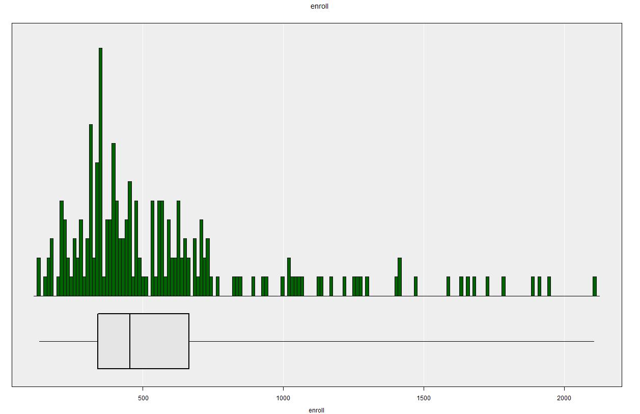
If we load the apisrs dataset note that it actually already has a population size column included, named fpc. If we specify this as the population size variable and then choose the enroll variable the default plot changes from a box+dot plot to a boxplot+histogram.
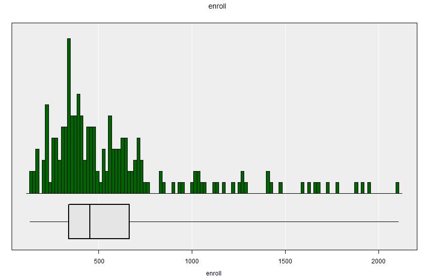
apisrs dataset - including the finite population correction.Get Summary reports details of the population size, and instead of just reporting single values for the variable’s characteristics (mean, standard deviation, median, quartiles) it repors these values as estimates and also reports their standard errors.
====================================================================================================
                                  iNZight Summary - Survey Design
----------------------------------------------------------------------------------------------------
   Primary variable of interest: enroll (numeric)

   Total number of observations: 200
      Estimated population size: 6194
----------------------------------------------------------------------------------------------------
   Independent Sampling design
   survey::svydesign(id = ~ 1, fpc = ~ N, data = dataSet)
====================================================================================================

Summary of enroll:
------------------

Population estimates:

       25%   Median      75%     Mean       SD     Total   Est. Pop. Size   |   Sample Size   Min    Max
   339.000   453.00   664.00   584.61   393.45   3621074             6194   |           200   131   2106

Standard error of estimates:

     9.632    28.53    28.51    27.37    30.39    169520                0

Design effects:

                                 1.00                  1

====================================================================================================
This summary output gives the estimate not only of the population mean school size \(\widehat{\bar{Y}}=584.61\) but also the population total: \(\widehat{Y}=N\widehat{\bar{Y}}=3621074\): an estimate of the total population of all the schools in the population combined. The standard errors of these two estimates are given (\(30.39\) and \(169520\) respectively).
The RSE for the estimate of the mean is the ratio of the standard error to the estimate: \[\begin{eqnarray*} \mathbf{RSE}[\widehat{\bar{Y}}] &=& \frac{\mathbf{SE}[\widehat{\bar{Y}}]}{\widehat{\bar{Y}}} \end{eqnarray*}\] In the R Console:
> 27.27/584.61
[1] 0.0466465
The Design Effect (Deff) is the variance of the estimate divided by the variance that would have been achieved by using data from a SRSRWOR of the same sample size. So by definition the Deff for a SRSWOR is always 1.
The output of Get Inference looks very similar to before, except that the population size is given.
====================================================================================================
                               iNZight Inference using Normal Theory
----------------------------------------------------------------------------------------------------
   Primary variable of interest: enroll (numeric)

   Total number of observations: 200
      Estimated population size: 6194
----------------------------------------------------------------------------------------------------
   Independent Sampling design
   survey::svydesign(id = ~ 1, fpc = ~ N, data = dataSet)
====================================================================================================

Inference of enroll:
--------------------

Population Mean with 95% Confidence Interval

   Lower    Mean   Upper
     531   584.6   638.3


====================================================================================================
Note however that the although the estimated mean is the same as before (584.6) the confidence interval is just slightly narrower: it is now (531.0,638.3) whereas without specifying the population size it was (529.7, 584.6). This is due to the variance of an estimator of the mean with SRSWOR including the finite population correction (fpc): \[\begin{eqnarray*} \text{Var}[\widehat{\bar{Y}}] &=& \left(1-\frac{n}{N}\right)\frac{S_Y^2}{n} \end{eqnarray*}\] and the fpc factor \((1-n/N)\) reduces the variance, thereby reducing the margin of error.
A confidence interval for the population total can be computed using the R Console by multiplying the confidence interval for the mean by the population size \(N=6194\):
> 6194*c(531, 638.3)
[1] 3.289014\times 10^{6}, 3.9536302\times 10^{6}
3.5.2 Example - Single categorical variable
Now look at the School Type variable stype:
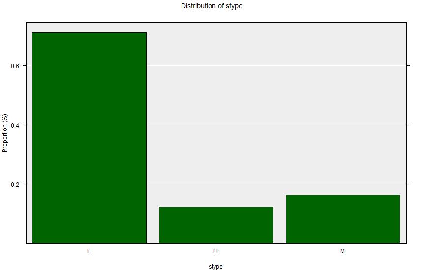
apisrs dataset - including the finite population correction.Summary output:
====================================================================================================
                                  iNZight Summary - Survey Design
----------------------------------------------------------------------------------------------------
   Primary variable of interest: stype (categorical)

   Total number of observations: 200
      Estimated population size: 6194
----------------------------------------------------------------------------------------------------
   Independent Sampling design
   survey::svydesign(id = ~ 1, fpc = ~ fpc, data = dataSet)
====================================================================================================

Summary of the distribution of stype:
-------------------------------------

Population Estimates:

                          E        H        M   Total
            Count      4398      774     1022    6194

          Percent    71.00%   12.50%   16.50%    100%
          std err     3.16%    2.31%    2.59%

   Design effects      1.00     1.00     1.00

====================================================================================================
Inference Output
====================================================================================================
                               iNZight Inference using Normal Theory
----------------------------------------------------------------------------------------------------
   Primary variable of interest: stype (categorical)

   Total number of observations: 200
      Estimated population size: 6194
----------------------------------------------------------------------------------------------------
   Independent Sampling design
   survey::svydesign(id = ~ 1, fpc = ~ fpc, data = dataSet)
====================================================================================================

Inference of the distribution of stype:
---------------------------------------

Estimated Population Proportions with 95% Confidence Interval

        Lower   Estimate   Upper
   E   0.6480      0.710   0.772
   H   0.0798      0.125   0.170
   M   0.1143      0.165   0.216


### Differences in proportions of stype
    (col group - row group)

Estimates

           E       H
   H   0.585
   M   0.545   -0.04

95% Confidence Intervals

            E          H
   H   0.5636
       0.6063
   M   0.5219   -0.05634
       0.5681   -0.02366


====================================================================================================
3.6 Two-variable analyses
The procedure for two variables with a SRSWOR design are the same as they are without a sample design. The output is slightly different - in particular for estimated counts of categorical variables: they are estimates of population total counts, and not simply sample counts.
3.6.1 Two numerical variables
Here we investigate the relationship between overall school academic performance (api00) and proportion of children receiving school meals (meals) in the apisrs data set.
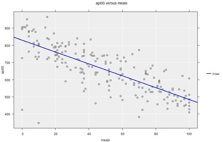
The Summary Output looks similar to the standard output, except that in addition to the correlation coefficient it also gives the coefficients for a linear regression fit. The Inference output also gives confidence intervals for those coefficients.
Summary Output:
====================================================================================================
                                  iNZight Summary - Survey Design
----------------------------------------------------------------------------------------------------
        Response/outcome variable: api00 (numeric)
   Predictor/explanatory variable: meals (numeric)

     Total number of observations: 200
        Estimated population size: 6194
----------------------------------------------------------------------------------------------------
   Independent Sampling design
   survey::svydesign(id = ~ 1, fpc = ~ fpc, data = dataSet)
====================================================================================================

Summary of api00 versus meals:
------------------------------

Summary of api00 versus meals:
------------------------------

Correlation: -0.78  (using Pearson's Correlation)

====================================================================================================
Inference Output:
====================================================================================================
                               iNZight Inference using Normal Theory
----------------------------------------------------------------------------------------------------
        Response/outcome variable: api00 (numeric)
   Predictor/explanatory variable: meals (numeric)

     Total number of observations: 200
        Estimated population size: 6194
----------------------------------------------------------------------------------------------------
   Independent Sampling design
   survey::svydesign(id = ~ 1, fpc = ~ fpc, data = dataSet)
====================================================================================================

Inference of api00 versus meals:
--------------------------------


Linear Trend Coefficients with 95% Confidence Intervals

               Estimate     Lower     Upper   p-value
   Intercept     829.37    802.22    856.52    <2e-16
       meals     -3.455   -3.8662   -3.0437    <2e-16


   p-values for the null hypothesis of no association, H0: beta = 0


====================================================================================================
3.6.2 One numerical and one categorical variable
Summary Output:
====================================================================================================
iNZight Summary - Survey Design
----------------------------------------------------------------------------------------------------
Primary variable of interest: api00 (numeric)
Secondary variable: stype (categorical)
Total number of observations: 200
Estimated population size: 6194
----------------------------------------------------------------------------------------------------
Independent Sampling design
survey::svydesign(id = ~ 1, fpc = ~ fpc, data = dataSet)
====================================================================================================
Summary of api00 by stype:
--------------------------
Population estimates:
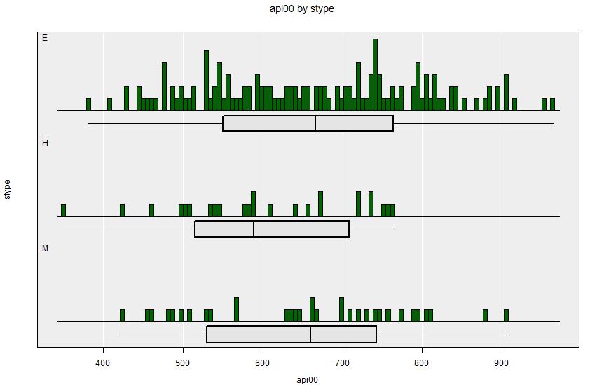
25% Median 75% Mean SD Total Est. Pop. Size | Sample Size Min Max
E 550.50 666.00 763.50 666.1408 135.73 2929514.240 4397.7 | 142 382 965
H 515.00 589.00 708.50 605.3600 113.46 468699.980 774.2 | 25 348 764
M 530.25 660.00 742.75 654.2727 129.11 668673.270 1022.0 | 33 425 905
Standard error of estimates:
E 13.91 19.63 15.54 11.1935 5.90 139532.264 196.0
H 39.56 33.05 34.43 21.9266 12.90 88125.597 142.8
M 41.11 37.92 25.31 21.8261 11.41 107242.153 160.3
Design effects:
E 0.9979 8.018
H 0.9648 25.998
M 0.9746 22.526
====================================================================================================Inference Output:
====================================================================================================
iNZight Inference using Normal Theory
----------------------------------------------------------------------------------------------------
Primary variable of interest: api00 (numeric)
Secondary variable: stype (categorical)
Total number of observations: 200
Estimated population size: 6194
----------------------------------------------------------------------------------------------------
Independent Sampling design
survey::svydesign(id = ~ 1, fpc = ~ fpc, data = dataSet)
====================================================================================================
Inference of api00 by stype:
----------------------------
Population Means with 95% Confidence Intervals
Lower Mean Upper
E 644.2 666.1 688.1
H 562.4 605.4 648.3
M 611.5 654.3 697.1
Wald test for stype (ANOVA equivalent for survey design)
F = 3.0482, df = 2 and 197, p-value = 0.04969
Null Hypothesis: true group means are all equal
Alternative Hypothesis: true group means are not all equal
### Difference in mean api00 between stype groups
(col group - row group)
Estimates
E H
H 60.78
M 11.87 -48.91
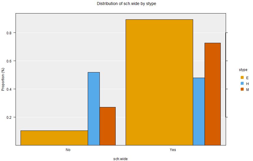
====================================================================================================3.6.3 Two categorical variables
 Summary Output:
====================================================================================================
                                  iNZight Summary - Survey Design
----------------------------------------------------------------------------------------------------
   Primary variable of interest: sch.wide (categorical)
             Secondary variable: stype (categorical)

   Total number of observations: 200
      Estimated population size: 6194
----------------------------------------------------------------------------------------------------
   Independent Sampling design
   survey::svydesign(id = ~ 1, fpc = ~ fpc, data = dataSet)
====================================================================================================

Summary of the distribution of sch.wide (columns) by stype (rows):
------------------------------------------------------------------

Table of Estimated Population Counts:

        No    Yes   Row Total
   E   465   3933        4398
   H   403    372         775
   M   279    743        1022

Table of Estimated Population Percentages:

          No     Yes   Total   Row N
   E   10.6%   89.4%    100%    4398
   H     52%     48%    100%     775
   M   27.3%   72.7%    100%    1022

Standard error of estimated percentages:

          No     Yes
   E   2.544   2.544
   H   9.854   9.854
   M   7.646   7.646

Design effects:

          No     Yes
   E   0.998   0.998
   H   0.965   0.965
   M   0.975   0.975


====================================================================================================
Inference Output:
====================================================================================================
                               iNZight Inference using Normal Theory
----------------------------------------------------------------------------------------------------
   Primary variable of interest: sch.wide (categorical)
             Secondary variable: stype (categorical)

   Total number of observations: 200
      Estimated population size: 6194
----------------------------------------------------------------------------------------------------
   Independent Sampling design
   survey::svydesign(id = ~ 1, fpc = ~ fpc, data = dataSet)
====================================================================================================

Inference of the distribution of sch.wide (columns) by stype (rows):
--------------------------------------------------------------------

Estimated Proportions

          No     Yes   Row sums
   E   0.106   0.894          1
   H   0.520   0.480          1
   M   0.273   0.727          1

95% Confidence Intervals

           No     Yes
   E   0.0558   0.845
       0.1555   0.944
   H   0.3269   0.287
       0.7131   0.673
   M   0.1229   0.577
       0.4226   0.877

Chi-square test for equal distributions

   X^2 = 13.482, df = 2 and 398, p-value = 2.1606e-06

          Null Hypothesis: distribution of sch.wide does not depend on stype
   Alternative Hypothesis: distribution of sch.wide changes with stype


### Differences in proportions of stype with the specified sch.wide

  # Group differences between proportions with: sch.wide = No
    (col group - row group)

Estimates

            E         H
   H   0.4144
   M   0.1671   -0.2473

  # Group differences between proportions with: sch.wide = Yes
    (col group - row group)

Estimates

             E        H
   H   -0.4144
   M   -0.1671   0.2473


====================================================================================================
3.7 SRS With Replacement
In a Simple Random Sample With Replacement (SRSWR) the members of the population can be selected more than once. So when we select a sample of \(n\) units from a population of size \(N\) we may end up with some repeated units in our sample.
The sample weights in SRSWR are the same as in SRSWOR: \[ w_i = \frac{N}{n} \] however the variances of our estimates are slightly larger.
When specifying a SRSWR to iNZight we need need to calculate the weights \(w_i\) in a new column, and we give these to iNZight, rather than specifying the population size. We need to:
- add a column to the dataset with the weight \(w_i=N/n\) repeated in every entry of the column
- tell iNZight that the data should be treated as a SRSWR, and specifying the column with the weights
The weights can be calculated creating a new column by computing \(N/n\), and filling this in to every entry in a column.
So add a column for the weights:
Variables > Create new variables- Fill in the two boxes in the window that opens:
- in the left hand box replace
new.variablewith the name you’re giving the weight: e.g.weight - in the right hand box fill in the values \(N/n\): e.g.
6194/200for theapisrsdata set
- in the left hand box replace
- Click
SUBMIT
To tell iNZight to use this column:
Dataset > Survey Design > Specify Design- In the
Weighting variablebox choose the name of the weight variable - Click
OK
3.7.1 Example
Load the apisrs data set. Let’s treat this as a SRSWR from the population, and estimate the mean school size (enroll). This data set already has the weights calculated in the column pw, but calculate them as described above in a new column called weight using \(N=6194\) and \(n=200\). You should see you’ve created a column with values 30.97, just as is already in the pw column.
Then specify the design, using the weight column as the weighting variable - and leaving the finite population correction blank.
Now choose enroll as Variable 1, and we’ll get exactly the same histogram as when we were treating the data as a SRSWOR.
apisrs dataset - as a SRSWR (excluding the finite population correction).Get Summary gives Population estimates which are exactly the same (apart from some rounding error) as what we had in the SRSWOR case:
====================================================================================================

                                  iNZight Summary - Survey Design
----------------------------------------------------------------------------------------------------
   Primary variable of interest: enroll (numeric)

   Total number of observations: 200
      Estimated population size: 6194
----------------------------------------------------------------------------------------------------
   Independent Sampling design (with replacement)
   survey::svydesign(id = ~ 1, weights = ~ weight, data = dataSet)
====================================================================================================

Summary of enroll:
------------------

Population estimates:

       25%   Median      75%      Mean       SD         Total   Est. Pop. Size   |   Sample Size   Min    Max
   339.000    453.0   664.00   584.610   393.45   3621074.340             6194   |           200   131   2106


Standard error of estimates:

     9.776     29.8    28.92    27.821    30.89    172324.604                0

Design effects:

                                 1.033                  1.033


====================================================================================================
However the standard errors are all just slightly larger: e.g. the standard error of the mean is 27.82 rather than 27.37, and this is reflected in the Design effect being slightly greater than 1 (1.033) for SRSWR, as opposed to being (by definition) exactly 1 for SRSWOR.
Get Inference gives a confidence interval of \((530.1, 639.1)\) under SRSWR compared to the marginally narrower interval \((531.0, 638.3)\) under SRSWOR.
====================================================================================================
                               iNZight Inference using Normal Theory
----------------------------------------------------------------------------------------------------
   Primary variable of interest: enroll (numeric)

   Total number of observations: 200
      Estimated population size: 6194
----------------------------------------------------------------------------------------------------
   Independent Sampling design (with replacement)
   survey::svydesign(id = ~ 1, weights = ~ weight, data = dataSet)
====================================================================================================

Inference of enroll:
--------------------

Population Mean with 95% Confidence Interval

   Lower    Mean   Upper
   530.1   584.6   639.1


====================================================================================================
3.8 With Replacement Designs
In iNZight when specifying a design we specify either the finite population correction or the weighting variable. If we specify the finite population correction we are telling iNZight to treat the data as being sampled without replacement. If we specify the weighting variable we are telling iNZight to treat the data as if sampled with replacement.
If the sampling fraction (the sample size as a proportion of the population size) is low, then the difference between the two estimation methods won’t be important.
If a sample design is with replacement, then the data are of course collected only once from each unit, no matter how many times a unit is selected. The data simply get repeated in the dataset according to the number of times each unit is selected.
Designs with probability proportional to size with replacement (PPSWR) can be much much more efficient than simple random samples if the variable of interest is proportional to some size measure which is known for every population unit.
This manual concentrates on without replacement sampling, and in each case uses the finite population correction to specify the design.