Chapter 4 Stratified SRS
In a stratified sample the population is first divided into \(H\) groups, known as strata, using auxiliary information on the frame. Each unit \(i\) in the population on the frame is placed into one and only one stratum on the basis of a stratification variable, or variables, \(X_i\).
There are \(N_h\) units in stratum \(h\), and these stratum sizes add to the population size \[\begin{eqnarray*} N &=& \sum_{h=1}^H N_h \end{eqnarray*}\] The stratum fractions \[\begin{eqnarray*} F_h = \frac{N_h}{N} \end{eqnarray*}\] add up to 1: \[\begin{eqnarray*} \sum_{h=1}^H F_h &=& 1 \end{eqnarray*}\]
In a stratified SRS we independently draw \(n_h\) units by SRSWOR from each stratum \(h=1,\ldots,H\). The sample weights of units in stratum \(h\) are \[\begin{eqnarray*} w_h = \frac{N_h}{n_h} \end{eqnarray*}\] The total sample size is \[\begin{eqnarray*} n &=& \sum_{h=1}^H n_h \end{eqnarray*}\]
4.1 Specifying a Stratified SRSWOR design
In order for iNZight to carry out an appropriate analysis of a Stratified SRSWOR, we need to identify which units in the sample come from which stratum, and we need to specify the stratum sizes \(N_h\). In iNZight this means
- adding a column to the dataset with the label \(h\) of the stratum to which each sample unit belongs, and then
- adding a column to the dataset with the stratum size \(N_h\) associated with the stratum to which the sample unit belongs, and then
- telling iNZight that the data should be treated as a Stratified SRSWOR, and specifying the columns with the stratum labels and stratum sizes.
We’ll assume that the two extra columns are already in the data set under consideration.
To tell iNZight to use these columns:
Dataset > Survey Design > Specify Design- In the
Strata variablesbox choose the name of the stratum label variable - In the
Finite population correctionbox choose the name of the population size variable - Click
OK
Note that we can clear the specification of a sample design just by going
Dataset > Survey Design > Remove Design
4.2 Example
In the apistrat data set in the example data supplied with iNZight in the survey package there is a stratified SRS of California Schools. The sample is stratified by School Type (stype), and the stratum sizes \(N_h\) are listed in the column fpc. There are \(H=3\) School Types (\(h=1=\)E=Elementary, \(h=2=\)H=High and \(h=3=\)M=Middle: note that these are always presented in graphs and output in alphabetical order: Elementary then High then Middle, even though the logical order would be E, M then H).
Before specifying any Survey Design, Get Summary on the variable stype shows that there are \(n_1=100\) Elementary Schools, \(n_2=50\) High Schools and \(n_3=50\) Middle Schools in the sample, and these are respectively 50%, 25% and 25% of the sample.
====================================================================================================
                                          iNZight Summary
----------------------------------------------------------------------------------------------------
   Primary variable of interest: stype (categorical)

   Total number of observations: 200
====================================================================================================

Summary of the distribution of stype:
-------------------------------------

                   E        H        M   Total
     Count       100       50       50     200
   Percent    50.00%   25.00%   25.00%    100%


====================================================================================================
Whereas after specifying the stratified sample design Get Summary shows us:
====================================================================================================
                                  iNZight Summary - Survey Design
----------------------------------------------------------------------------------------------------
   Primary variable of interest: stype (categorical)

   Total number of observations: 200
      Estimated population size: 6194
----------------------------------------------------------------------------------------------------
   Stratified Independent Sampling design
   survey::svydesign(id = ~ 1, strata = ~ stype, fpc = ~ fpc, data = dataSet)
====================================================================================================

Summary of the distribution of stype:
-------------------------------------

Population Estimates:

                          E        H        M   Total
            Count      4421      755     1018    6194

          Percent    71.38%   12.19%   16.44%    100%
          std err     0.00%    0.00%    0.00%

   Design effects      0.00     0.00     0.00

====================================================================================================
This output shows us the ‘estimated’ stratum sizes \(N_1=4421\), \(N_2=755\) and \(N_3=1018\), adding up to the total population \(N=6194\) - they have zero sampling error because in they are known with certainty (and their Deffs are therefore also zero). The stratum fractions \(F_1=0.7138\), \(F_2=0.1219\) and \(F_3=0.1644\) add up to 1.
4.3 Within stratum properties
Means, standard deviations and totals within strata can be estimated by selecting the variable of interest as Variable 1 and the stratification variable as Variable 2.
4.3.1 Example
In the apistrat dataset we can find the within stratum propoerties of the enroll variable by setting enroll as Variable 1 and stype as Variable 2.
The Summary output is:
====================================================================================================
                                  iNZight Summary - Survey Design
----------------------------------------------------------------------------------------------------
   Primary variable of interest: enroll (numeric)
             Secondary variable: stype (categorical)

   Total number of observations: 200
      Estimated population size: 6194
----------------------------------------------------------------------------------------------------
   Stratified Independent Sampling design
   survey::svydesign(id = ~ 1, strata = ~ stype, fpc = ~ fpc, data = dataSet)
====================================================================================================

Summary of enroll by stype:
---------------------------

Population estimates:

          25%    Median       75%      Mean       SD     Total   Est. Pop. Size   |   Sample Size   Min    Max
   E   298.00    385.00    522.00    416.78   166.06   1842584             4421   |           100   143   1112
   H   688.50   1377.00   1777.00   1320.70   671.07    997128              755   |            50   119   3156
   M   546.50    739.00    983.00    832.48   395.36    847465             1018   |            50   179   2171

Standard error of estimates:

   E    17.17     21.74     34.95     16.42    16.45     72581                0
   H   135.83    127.34    113.06     91.71    60.49     69239                0
   M    53.25     64.17     72.69     54.52    57.56     55503                0

Design effects:

   E                                   1.00                  1
   H                                   1.00                  1
   M                                   1.00                  1


====================================================================================================
The within-stratum Deffs are all 1, because these are just SRSWORs within strata.
4.4 Estimation
Estimation for stratified designs proceeds in exactly the same way as with SRSWOR, but with the difference that there is a stratified design.
For example, in the apistrat data set we can fit a regression model where academic performance api00 is predicted by meals: i.e. the proportion of children receiving school meals.
Under a stratified design, each observation has a weight that is determined by the stratum \(h\) that it belongs to (\(w_h=N_h/n_h\)), and the scatter plot shows these different weights by drawing plot symbols that are proportional to the size of the weight.
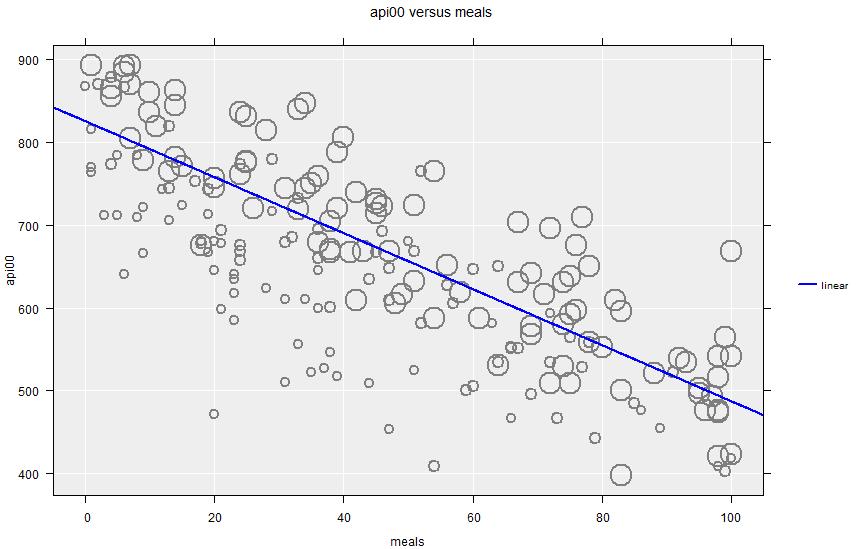
The Summary output looks very similar to the SRSWOR output, showing a linear relationship:
====================================================================================================
                                  iNZight Summary - Survey Design
----------------------------------------------------------------------------------------------------
        Response/outcome variable: api00 (numeric)
   Predictor/explanatory variable: meals (numeric)

     Total number of observations: 200
        Estimated population size: 6194
----------------------------------------------------------------------------------------------------
   Stratified Independent Sampling design
   survey::svydesign(id = ~ 1, strata = ~ stype, fpc = ~ fpc, data = dataSet)
====================================================================================================

Summary of api00 versus meals:
------------------------------

Correlation: -0.81  (using Pearson's Correlation)

====================================================================================================
The Inference output allows for a linear, quadratic or cubic fit, and again shows a similar output to the one we see under SRS.
====================================================================================================
                               iNZight Inference using Normal Theory
----------------------------------------------------------------------------------------------------
        Response/outcome variable: api00 (numeric)
   Predictor/explanatory variable: meals (numeric)

     Total number of observations: 200
        Estimated population size: 6194
----------------------------------------------------------------------------------------------------
   Stratified Independent Sampling design
   survey::svydesign(id = ~ 1, strata = ~ stype, fpc = ~ fpc, data = dataSet)
====================================================================================================

Inference of api00 versus meals:
--------------------------------


Linear Trend Coefficients with 95% Confidence Intervals

               Estimate    Lower     Upper   p-value
   Intercept     825.43   808.88    841.97    <2e-16
       meals    -3.3829   -3.712   -3.0538    <2e-16


   p-values for the null hypothesis of no association, H0: beta = 0


====================================================================================================
4.5 Sub-domain estimation
In sample surveys we often want to make estimates in sub-domains: namely estimates of a parameter within subsets of the population, those subsets being defined by variables we have measured in the data set. These variables are usually categorical (e.g. region, sex) but can also be numerical variables grouped into ranges (e.g. age group, income band).
Although one set of sub-domains of interest usually coincide with the strata in a stratified design, the sub-domains can be any set of subgroups, and don’t need to nest inside the strata. The only important consideration is that the sample size in the subdomains are large enough for reliable estimates to be formed within them.
In iNZight specifying only categorical variables as the last variables in the list will mean that the earlier variables are analysed and reported in groupings defined by those latter variables.
4.5.1 Example - Regression in sub-domains
In the apistrat data set we can do a regression of academic performance (api00) on percentage of school meals (meals) by specifying api00 as Variable 1 and meals as Variable 2. If we further specify sch.wide as a third variable (indicating the meeting of School Wide growth targets), then the regression is carried out separately in each domain.
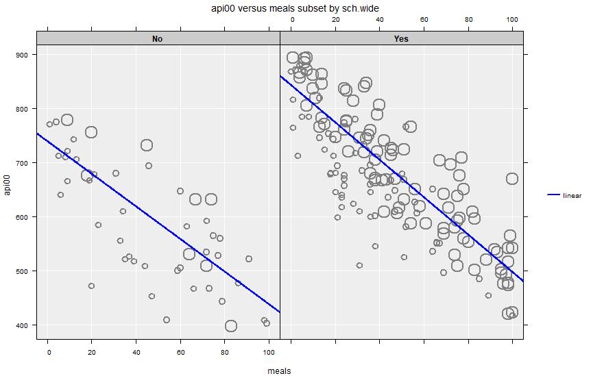
The Inference output in that case is
====================================================================================================
                               iNZight Inference using Normal Theory
----------------------------------------------------------------------------------------------------
        Response/outcome variable: api00 (numeric)
   Predictor/explanatory variable: meals (numeric)

                        Subset by: sch.wide

     Total number of observations: 200
        Estimated population size: 6194
----------------------------------------------------------------------------------------------------
   Stratified Independent Sampling design
   survey::svydesign(id = ~ 1, strata = ~ stype, fpc = ~ fpc, data = dataSet)
====================================================================================================

----------------------------------------------------------------------------------------------------
Inference of api00 versus meals, for sch.wide = No:
---------------------------------------------------


Linear Trend Coefficients with 95% Confidence Intervals

               Estimate     Lower     Upper   p-value
   Intercept     739.24     701.9    776.59    <2e-16
       meals    -3.0068   -3.7008   -2.3129     8e-11


   p-values for the null hypothesis of no association, H0: beta = 0

----------------------------------------------------------------------------------------------------
Inference of api00 versus meals, for sch.wide = Yes:
----------------------------------------------------


Linear Trend Coefficients with 95% Confidence Intervals

               Estimate     Lower     Upper   p-value
   Intercept      842.8    826.14    859.47    <2e-16
       meals    -3.4503   -3.7804   -3.1203    <2e-16


   p-values for the null hypothesis of no association, H0: beta = 0


====================================================================================================
The analysis is repeated, once for sch.wide = No and then for sch.wide = Yes. Of interest here is that the slope is very similar in the two subsets (both have slopes around -3) even though the intercepts are very different.