Temperature data from spring of 1996 and of 1999 have been analysed to obtain the amplitudes and relative phases of those oscillations with a period of one day, and the results are displayed in figures 6, 7, 8, and 9. Note that the scaled depth z=1 corresponds to 2m.
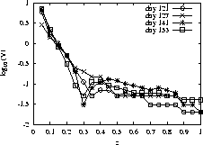
Figure 6: Amplitudes of temperature
oscillations observed in spring of 1996. The day number refers
to the numbering used in the temperature data (1),
and indicates
the day near which the data was obtained.
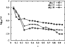
Figure 7: Amplitudes of temperature
oscillations observed in spring of 1999. The day number refers
to the numbering used in the temperature data
(2),
and indicates
the day near which the data was obtained.
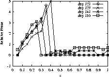
Figure 8: Relative phases of
temperature oscillations
observed during spring of 1996. The day number refers
to the numbering used in the temperature data (1),
and indicates
the day near which the data was obtained.
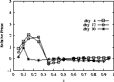
Figure 9: Relative phases of temperature oscillations
observed during spring of 1999. The day number refers
to the numbering used in the temperature data
(2),
and indicates
the day near which the data was obtained.
The phases plotted are relative phases, with deep phases
arbitrarily set to zero, and with the allowed range of phase being
from zero to ![]() .
.
A two-layer structure or behaviour is clearly evident in the data, and
correlates well with what is observed in the numerical solutions. In
a shallow layer we call the conductive region, up to ![]() 0.8m deep
(
0.8m deep
( ![]() ), amplitudes decrease most rapidly, and the phase
varies approximately linearly with depth, consistent with (damped)
travelling waves of constant velocity. Temperature changes in this
conductive region are driven by the rapid changes in amplitude
associated with rapid changes in the solar driving term P.
), amplitudes decrease most rapidly, and the phase
varies approximately linearly with depth, consistent with (damped)
travelling waves of constant velocity. Temperature changes in this
conductive region are driven by the rapid changes in amplitude
associated with rapid changes in the solar driving term P.
The fact that much of the incoming solar radiation is absorbed in a shallow layer is well-known, and Zeebe and others (1996) use this to justify accommodating the effects of longer wavelengths in their boundary condition at the surface of the sea ice. What is perhaps surprising here is the large thermal footprint of the shallow layer, in that the travelling waves originating there can be seen to penetrate nearly 1 m into the sea ice before their amplitudes diminish to the size of the deeper layer amplitudes. The size of this footprint is seen to be reduced after warming the ice, when deep amplitudes are increased, particularly in figure 7.
In the deeper layer, data amplitudes decrease relatively slowly, and
phase is almost constant at ![]() . This corresponds physically to
simple volumetric solar heating with negligible conductive heat flow.
We observe that after the ice warms to near -5
. This corresponds physically to
simple volumetric solar heating with negligible conductive heat flow.
We observe that after the ice warms to near -5 ![]() C, deep
amplitudes increase, and the conductive region shrinks in size. This
effect is particularly apparent in figures 7
and 9, with day 30 amplitudes raised at depth
compared with the other deep amplitudes, and the conductive region
from the phase plot for day 30 noticeably smaller. Note that day 30
was in a period of significant warming for the 1999 data
(figure 2).
C, deep
amplitudes increase, and the conductive region shrinks in size. This
effect is particularly apparent in figures 7
and 9, with day 30 amplitudes raised at depth
compared with the other deep amplitudes, and the conductive region
from the phase plot for day 30 noticeably smaller. Note that day 30
was in a period of significant warming for the 1999 data
(figure 2).