Numerical solutions have been obtained for equation (14),
using Mathematica and a standard numerical procedure called the shooting
method (e.g., Press and others, 1986). Plots of numerical solutions appear in
figures 4 and 5. The two
major line groupings in the amplitude plot correspond to the two extreme
choices of case b and case c for P(z). The effect of changing from case b
to case c is not as dramatic in the phase curves. The muliple clusters of
lines within these two major groupings correspond to different choices of the
parameters
![]() and
and ![]() . Numerical solutions can be seen to be relatively
insensitive to these parameters, depending mainly on the scattering
properties of the sea ice (that is, on case b and case c). The values
actually used for
. Numerical solutions can be seen to be relatively
insensitive to these parameters, depending mainly on the scattering
properties of the sea ice (that is, on case b and case c). The values
actually used for ![]() are 0,1,10,100, and 1000. The value 1000
was found to give results indistinguishable from infinity, so the full
range of surface boundary conditions are allowed for, from fully
insulating to perfect thermal contact. Values chosen for the surface
air temperature
are 0,1,10,100, and 1000. The value 1000
was found to give results indistinguishable from infinity, so the full
range of surface boundary conditions are allowed for, from fully
insulating to perfect thermal contact. Values chosen for the surface
air temperature ![]() range from -5
range from -5 ![]() C to -20
C to -20 ![]() C.
C.
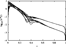
Figure 4: Amplitudes of temperature
oscillations obtained from numerical model solutions. The
different curves correspond to different parameter values as explained in
the text.
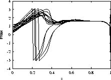
Figure 5: Phases of temperature
oscillations obtained from numerical model solutions. The
different curves correspond to different parameter values as explained in
the text.
Of some interest in the numerical solutions is the appearance of a
solid-state greenhouse effect, with the maximum in temperature
oscillation amplitude appearing at a depth of about 0.1 m beneath the
surface of the ice, for values of ![]() that correspond to good
thermal contact with the air. This is not observed in the data, since the
spacing of the thermistors is not close enough near the ice surface to resolve
it.
that correspond to good
thermal contact with the air. This is not observed in the data, since the
spacing of the thermistors is not close enough near the ice surface to resolve
it.