The optical energy absorbed in unit volume at any depth z in the ice is given by the product of the average radiance and the absorption coefficient. However the average radiance is not easily determined within the very successful Monte Carlo models we have developed on the basis of light spreading measurements. We have thus adapted these models to simulate the absorption process.
The core element in the Monte Carlo models is the tracing of many
randomly scattered light paths for rays impinging on the surface. The
effects of scattering are modeled by a depth-dependent scattering
length (mean-free-path) whose magnitude and depth dependence are
chosen to reproduce experimentally-determined beam-spreading profiles
(Haines and others, 1997). In the present case, where we wish to
simulate the heat absorbed in the ice, we follow the paths through
many layers of width ![]() centred at depths
centred at depths ![]() ,
and record for each traverse j of a ray through that layer the path
length
,
and record for each traverse j of a ray through that layer the path
length ![]() spent in the layer, binned by
the total path
spent in the layer, binned by
the total path ![]() that
the ray has followed before reaching that level. Then the absorbed
power per unit volume at that depth due to a flux
that
the ray has followed before reaching that level. Then the absorbed
power per unit volume at that depth due to a flux ![]() falling on the surface in wavelength bands
falling on the surface in wavelength bands ![]() to
to
![]() , and summed over all wavelengths, is
, and summed over all wavelengths, is
where N is the number of rays used in the Monte Carlo model, and
![]() is the absorption coefficient for pure ice in the
wavelength band
is the absorption coefficient for pure ice in the
wavelength band ![]() to
to
![]() .
The wavelength range used is 300-1400 nm. The
specific models, specified by the depth-dependent scattering length,
include three of those determined for McMurdo Sound first-year ice
(Haines and others, 1997). We note that they all
display a strongly scattering surface layer and a more weakly
scattering interior, and these features will be seen below to influence
the light absorption profiles. Such a two-layer structure is also
apparent in studies of Arctic first year sea ice (eg, Perovich and
others, 1998).
.
The wavelength range used is 300-1400 nm. The
specific models, specified by the depth-dependent scattering length,
include three of those determined for McMurdo Sound first-year ice
(Haines and others, 1997). We note that they all
display a strongly scattering surface layer and a more weakly
scattering interior, and these features will be seen below to influence
the light absorption profiles. Such a two-layer structure is also
apparent in studies of Arctic first year sea ice (eg, Perovich and
others, 1998).
The base ten logarithms of the resulting power densities are plotted against depth in figure 3. The models used range from the most transparent (c), through an intermediate case (a), to the most opaque or turbid (b) of those developed by Haines and others (1997). The powers are for midday during spring, and are used as an estimate of the peak-to-peak variation of solar power. They are used in the distributed source term in the heat conduction modelling in the next section, and they are the most important factor in determining the amplitudes of temperature oscillations in the ice due to solar radiation penetration.
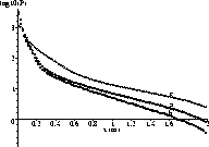
Figure 3: The base ten logarithm
of solar power absorbed per unit
volume (J m ![]() ), versus depth in
the sea ice, calculated by Monte Carlo scattering, and using
scattering lengths fitted to 1986 experiments. The labels a,b,c on
the
curves correspond to cases 86A, 86B, and 86C respectively, used
by Haines and others (1997). The power is that at midday on a
typical spring day in McMurdo Sound.
), versus depth in
the sea ice, calculated by Monte Carlo scattering, and using
scattering lengths fitted to 1986 experiments. The labels a,b,c on
the
curves correspond to cases 86A, 86B, and 86C respectively, used
by Haines and others (1997). The power is that at midday on a
typical spring day in McMurdo Sound.