Goodness-of-Fit Algorithms

Goodness-of-Fit Algorithms

TABLE OF CONTENTS

• Introduction to this web page
• Distribution-free goodness-of-fit testing of exponentiality
• Calculation of Kolmogorov-Smirnov statistics
• R code

---

Introduction

These web pages provide some information and results on goodness-of-fit tests for exponentiality, as described in Haywood and Khmaladze (2005). Algorithms using the R statistical software are also described. We wish to test the hypothesis that the sample {X_i}ⁿ_i=1 is from an exponential distribution or, more formally, that the i.i.d. random variables {X_i}ⁿ_i=1 all have exponential distribution function F(x)=1-e^-λx for some unknown (or unspecified) value of λ>0.

Distribution-free goodness-of-fit testing of exponentiality

We suggest as test statistics functionals from the transformed empirical process

w_n(x) = √n[P_n(x) - K_n(x, P_n)]

where P_n(x) is the empirical distribution function of the observations and K_n(x, P_n) is its compensator. In the case of exponential distributions the compensator has the very simple form:


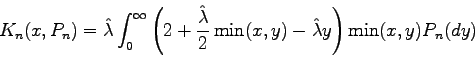
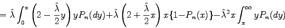
or

Calculation of Kolmogorov-Smirnov statistics for testing exponentiality via Khmaladze transformation

Calculation of the Kolmogorov-Smirnov statistics

becomes easy and yet exact, since within each interval (X_(j), X_(j+1)) formed by adjacent order statistics the compensator K_n(x, P_n) is a quadratic function in x.

A background note explains the theory behind these calculations. In the following calculations and code, the parameter lambda is estimated by . The code in R (see The R Project for Statistical Computing) for calculation of all three statistics takes the form of a series of functions shown below. We also show an example of K_n(x,P_n) for a small sample size (n=5).

The R code

Each of the following R functions is vectorised in x.

nPn <- function(x, X, n) {
  # returns n*Pn(x) given data X
  lx <- length(x)
  numi <- numeric(lx)
  for (i in 1:lx)
    numi[i] <- sum(X <= x[i])
  return(numi)
}

K <- function(x, X, n) {
  # returns K(x, Pn(x)) given data X
  lhat <- 1/(mean(X) + 1)
  cX <- c(0, cumsum(X))
  cX2 <- c(0, cumsum(X**2))
  crX <- cX[n+1] - cX
  if ((lx <- length(x)) > 0) {
    whichn <- nPn(x, X, n) + 1
  }
  return(lhat/n*(2*cX[whichn] - lhat/2*cX2[whichn]) +
    lhat*(2 + lhat/2*x)*x*(1 - nPn(x, X, n)/n) -
    lhat**2*x/n*crX[whichn])
}

x0 <- function(X, n) {
  # returns the value of x0 for each interval of X,
  # or the interval boundary value closest to it
  cX <- cumsum(X)
  crX <- cX[n] - cX[-n]
  invlhat <- mean(X) + 1
  maxloc <- crX/((n - 1):1) - 2*invlhat
  return(pmin(X[-1], pmax(X[-n], maxloc)))
}

findSup <- function(X) {
  n <- length(X)
  ivec <- 1:n
  ishort <- 1:(n - 1)
  dplus <- max(ivec/n - K(X, X, n), ishort/n - K(x0(X, n), X, n))
  dminus <- -min((ivec - 1)/n -  K(X, X, n))
  return(list(dplus=dplus, dminus=dminus, d=max(dplus, dminus)))
}

The Kolmogorov-Smirnov statistic is found by typing the R command:

findSup(sort(mydata))

where mydata is the dataset of interest.

In the small sample graph [PDF, 37KB], the compensator K_n(x, P_n) in black has one interval where it attains its minimum within the two endpoints of the interval (rather than at one of the endpoints). This is actually a rare occurrence, occurring perhaps only once in 1000 intervals.