The real world is fully of uncertainties. The source of uncertainties can be from true uncertainty (e.g., the outcome of flipping a coin is unknown in advance), theoretical ignorance (e.g., lack of knowledge in medical diagnosis), laziness (e.g., do not want to collect useful information such as doing survey to understand customers' opinion about a product), practical ignorance (e.g., missing information due to security/privacy), etc.
This lecture will introduce the basics of reasoning under uncertainty.
We can describe the uncertainty as random events/propositions. Following are some examples of propositions:
A basic proposition can be presented by a random variable, which can take values from its domain. In the above example 1, the random variable is weather
, whose domain is {rainy, sunny, cloudy}
. In the example 2, the random variable is US_stock_return
, whose domain is all the real values $\mathbb{R}$.
For the sake of simplicity, here we only consider finite discrete domains. We convert continuous domains to finite discrete ones by discretisation. For example, in the above example 2, we can discretise the continuous domain $\mathbb{R}$ into {very poor, poor, ok, good, very good}
, where
In other words, a basic proposition $A$ can be presented as
$$A: X = x, $$where $X$ is a random variable in $A$, and $x$ is a value from its domain. Examples include weather = rainy
and US_stock_return = good
.
A composite event/proposition combines one or more basic events/propositions with logic operators. Given two propositions $A$ and $B$,
In the above example 2, the proposition "$A$: The US stock market return will be at least 10% in 2022" is a composite proposition that can be written as
US_stock_return = good
$\mathsf{OR}$ US_stock_return = very good
.Probability is to measure how likely an event occur, or a proposition is true. Given an event/proposition $A$, the probability for $A$ to be true is denoted as $P(A)$. The probability has the following axioms.
If we roll a fair die with all the six numbers occur with the same probability, we know that the probability of each number is as follows:
Die | 1 | 2 | 3 | 4 | 5 | 6 |
---|---|---|---|---|---|---|
Prob | 1/6 | 1/6 | 1/6 | 1/6 | 1/6 | 1/6 |
QUESTION: If we roll two fair dice, What is the probability that the total number of the two dice is 11?
For a composite proposition with the $\mathsf{AND}$ logic, e.g., $A\ \mathsf{AND}\ B$, the probability is also called the joint probability $P(A,B)$.
$$ P(A,B) = P(A\ \mathsf{AND}\ B). $$In other words, the joint probability $P(A,B)$ means the probability that $A$ and $B$ are both true.
The unconditional/prior probability reflects the belief in propositions in the absence of any other information/evidence. Examples include:
The conditional probability is the upldated belief in propositions given some more information/evidence. Below are possible examples:
We can see that the conditional probability of a proposition can be dramatically different from its prior probability. In other words, conditions/evidence can greatly change the belief of propositions.
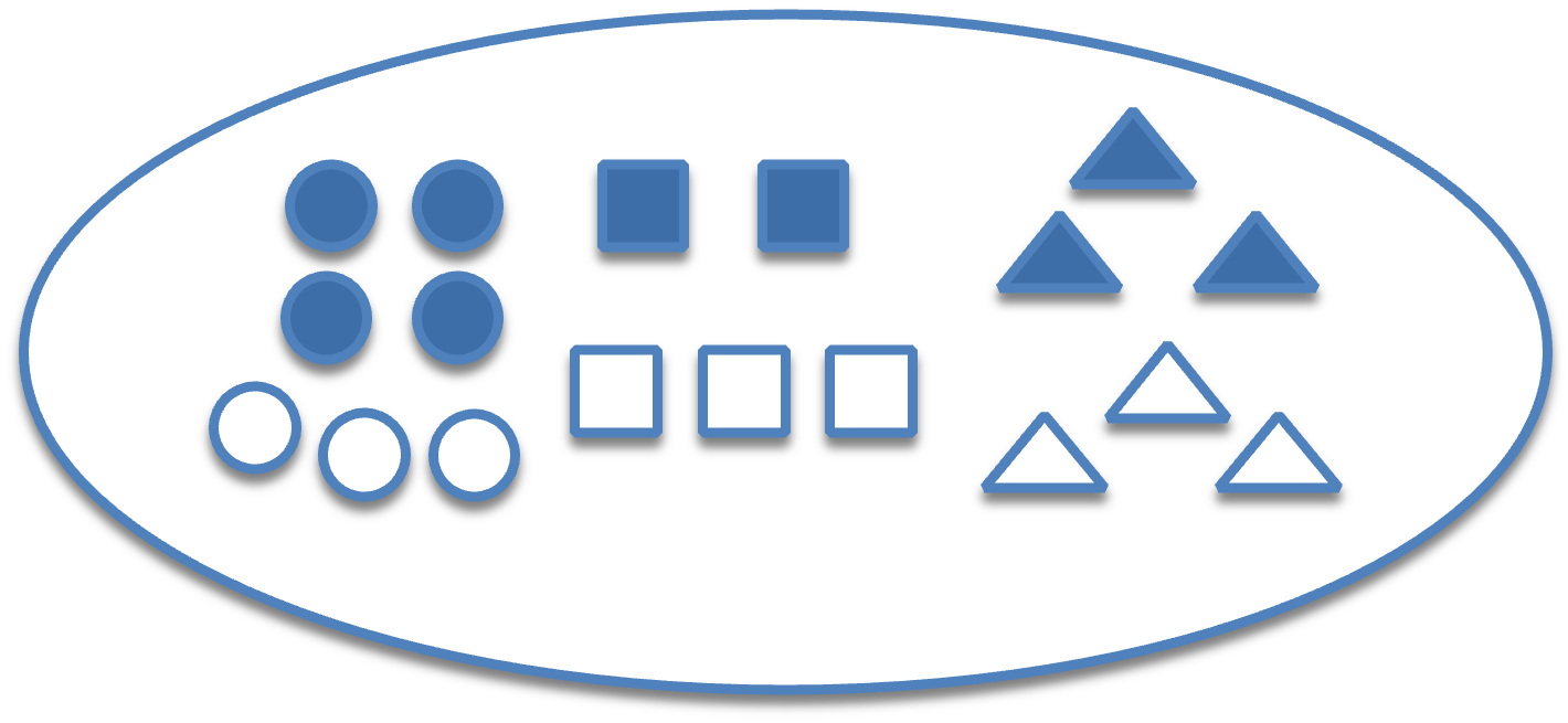
In the above example, there are 18 objects in a bag with different colours and shapes. The numbers of objects with each colour and shape are given below.
Circle | Square | Triangle | Total | |
---|---|---|---|---|
Blue | 4 | 2 | 3 | 9 |
White | 3 | 3 | 3 | 9 |
Total | 7 | 5 | 6 | 18 |
If we randomly pick an object from the bag, the colour
and shape
of the picked object are random variables.
We can calculate the probabilities by counting the numbers. For example,
blue
object is 9/18 (there are 9 blue objects out of the 18 objects in total), i.e., P(blue) = 9/18
.white
and square
object is 3/18 (there are 3 objects with white colour and square shape), i.e., P(white, square) = 3/18
.circle
shape, given that we have seen its colour is blue
, is 4/9 (there are 4 objects with circle shape among the 9 objects with blue colour), i.e., P(circle | blue) = 4/9
.Below are the three commonly used probability rules.
Given two propositions $A$ and $B$, we have
$$ P(A,B) = P(A) * P(B | A). $$The product rule can be explained by establishing the beliefs of $A$ and $B$ in two different ways: parallel and sequential.
Since we will reach the same belief through either parallel or sequential way, we have $P(A,B) = P(A) * P(B | A)$.
In the sequential way, we can also establish our belief for $B$ first, and then $A$ given $B$. Then we can obtain $P(A,B) = P(B) * P(A | B)$. In other words, the product rule works for any order of random variables.
We can further extend the product rule from two propositions to any number of propositions. Given a list of propositions $A_1, A_2, \dots, A_n$, we have
$$ P(A_1, A_2, \dots, A_n) = P(A_1) * P(A_2 | A_1) * \dots * P(A_n | A_1, A_2, \dots, A_{n-1}). $$This is the famous chain rule) for probability.
Given two discrete random variables $X$ and $Y$, with their domains as $\Omega(X)$ and $\Omega(Y)$, then for each $x \in \Omega(X)$, we have
$$ P(X = x) = \sum_{y \in \Omega(Y)} P(X = x, Y = y). $$In other words, if we jointly consider a random variable $X$ with another random variable $Y$, then the marginal probability $P(X = x)$ is equivalent to the sum of its joint probabilities over all the possible $Y$ values.
For example, if we consider tomorrow's weather $X_{t+1}$ jointly with today's weather $X_t$, where there are three possible weathers $\{sunny, rainy, cloudy\}$, then we have
$$ \begin{aligned} P(X_{t+1} = sunny) & = P(X_{t+1} = sunny, X_t = sunny) \\ & + P(X_{t+1} = sunny, X_t = rainy) \\ & + P(X_{t+1} = sunny, X_t = cloudy) \end{aligned} $$$$ \begin{aligned} P(X_{t+1} = rainy) & = P(X_{t+1} = rainy, X_t = sunny) \\ & + P(X_{t+1} = rainy, X_t = rainy) \\ & + P(X_{t+1} = rainy, X_t = cloudy) \end{aligned} $$$$ \begin{aligned} P(X_{t+1} = cloudy) & = P(X_{t+1} = cloudy, X_t = sunny) \\ & + P(X_{t+1} = cloudy, X_t = rainy) \\ & + P(X_{t+1} = cloudy, X_t = cloudy) \end{aligned} $$We can further extend the sum rule from two random variables to any number of variables. Given random variables $X_1, X_2, \dots, X_m$ and $Y_1, Y_2, \dots, Y_n$, then for each $x_1 \in \Omega(X_1), x_2 \in \Omega(X_2), \dots x_m \in \Omega(X_m)$, we have
$$ P(X_1 = x_1, \dots, X_m = x_m) = \sum_{y_i \in \Omega(Y_i), i = 1, \dots, n} P(X_1 = x_1, \dots, X_m = x_m, Y_1 = y_1, \dots, Y_n = y_n). $$Given a discrete random variable $X$ with its domain $\Omega(X)$, we have
$$ \sum_{x = \Omega(X)} P(X) = 1. $$It is obvious that the random variable must take one of the values in its domain. Therefore, the probabilities of all the possible values should add up to 1 (100%).
The normalisation rule holds under any condition as well. Given any conditional proposition $A$, we have
$$ \sum_{x = \Omega(X)} P(X | A) = 1. $$In the above weather forecast example, the normalisation rule without condition can be written as:
$$ P(X_{t+1} = sunny) + P(X_{t+1} = rainy) + P(X_{t+1} = cloudy) = 1, $$Similarly, the normalisation rule under the condition $X_t = sunny$ can be written as:
$$ P(X_{t+1} = sunny | X_t = sunny) + P(X_{t+1} = rainy | X_t = sunny) + P(X_{t+1} = cloudy | X_t = sunny) = 1, $$Given two random variables $X$ and $Y$, if for any possible value $x \in \Omega(X)$, the probability $P(X = x)$ does not depend on the $Y$ value, then we call that $X$ and $Y$ are independent of each other, denoted as $X \perp Y$.
If two random variables $X$ and $Y$ are independent, then for each $x \in \Omega(X)$ and $y \in \Omega(Y)$, we have
$$ P(X = x | Y = y) = P(X = x). $$This is obvious by definition, since our belief on $P(X = x)$ does not change at all no matter whether we have information on $Y$ or not.
Similarly, we have
$$ P(Y = y | X = x) = P(Y = y). $$Further, combined with the product rule, we have
$$ P(X = x, Y = y) = P(X = x) * P(Y = y), $$For example, if we flip a fair coin twice, where the two outcome head
or tail
have the same probability of 0.5, then the outcome of the two flips are independent of each other. We have
For more variables, we say that $X_1, \dots, X_n$ are independent with each other, if
$$ P(X_1, \dots, X_n) = P(X_1) * \dots * P(X_n). $$The independence can also be conditional. Given random variables $X$, $Y$ and $Z$, we say that $X$ and $Y$ are conditionally independent given $Z$, if for each $x \in \Omega(X)$, $y \in \Omega(Y)$ and $z \in \Omega(Z)$, we have
$$ P(X = x, Y = y | Z = z) = P(X = x | Z = z) * P(Y = y | Z = z). $$We can see that the formula of conditional independence is obtained by adding the condition (e.g., $| Z = z)$ into each probability of the unconditional formula.
For more variables, we say that $X_1, \dots, X_n$ are independent given $Y_1, \dots, Y_m$, if
$$ P(X_1, \dots, X_n | Y_1, \dots, Y_m) = P(X_1 | Y_1, \dots, Y_m) * \dots * P(X_n | Y_1, \dots, Y_m). $$In this case study, we aim to forecast the weather in the future. The weather is denoted as random variable $X$, and its domain (possible weathers) is $\{Sunny, Rainy\}$.
For the weather tomorrow, denoted as $X_t$, the forecast says that it will be sunny with probability of 20%, and rainy with probability of 80% (obviously, they sum up to 100% due to normalisation rule). That is,
$$ P(X_t = sunny) = 0.2,\\ P(X_t = rainy) = 0.8. $$We also know that the weather tends to change smoothly over time. Thus, the weather for the day after tomorrow, denoted as $X_{t+1}$, depends on the weather tomorrow as follows.
In other words, we have
$$ P(X_{t+1} = sunny | X_t = sunny) = 0.6, \\ P(X_{t+1} = rainy | X_t = sunny) = 0.4, $$$$ P(X_{t+1} = sunny | X_t = rainy) = 0.3, \\ P(X_{t+1} = rainy | X_t = rainy) = 0.7. $$What is the probability that the day after tomorrow will be sunny?
The probability that the day after tomorrow will be sunny can be written as $P(X_{t+1} = sunny)$.
First, we can use the sum rule to take the weather tomorrow into consideration as follows:
$$ P(X_{t+1} = sunny) = P(X_{t+1} = sunny, X_t = sunny) + P(X_{t+1} = sunny, X_t = rainy). $$Then, for each term on the right hand side, we can use the product rule that considers $X_t$ first, and then $X_{t+1}$ given $X_t$. Specifically, we have
$$ P(X_{t+1} = sunny, X_t = sunny) = P(X_t = sunny) * P(X_{t+1} = sunny | P(X_t = sunny), \\ P(X_{t+1} = sunny, X_t = rainy) = P(X_t = rainy) * P(X_{t+1} = sunny | P(X_t = rainy). $$All the above probabilities on the right hand side are known from the forecast. Therefore, we have
$$ \begin{aligned} P(X_{t+1} = sunny, X_t = sunny) & = P(X_t = sunny) * P(X_{t+1} = sunny | P(X_t = sunny) \\ & = 0.2 \times 0.6 = 0.12, \end{aligned} $$$$ \begin{aligned} P(X_{t+1} = sunny, X_t = rainy) & = P(X_t = rainy) * P(X_{t+1} = sunny | P(X_t = rainy) \\ & = 0.8 \times 0.3 = 0.24. \end{aligned} $$Therefore, we have
$$ \begin{aligned} P(X_{t+1} = sunny) & = P(X_{t+1} = sunny, X_t = sunny) + P(X_{t+1} = sunny, X_t = rainy) \\ & = 0.12 + 0.24 = 0.36. \end{aligned} $$